Headless

Here's the problem I had to solve: my Differential Global Navigation Satellite System (GNSS) base station runs in "survey-in" mode for days in order to achieve a positioning resolution down to a few centimeters. This procedure takes so long that the Raspberry Pi 3B+, on which my gpstool software runs to process the output from the u-blox ZED-F9P GNSS module, is powered by an Uninterruptible Power Supply (UPS).

 (Click on any image to see a larger version.)

gpstool has a useful, simple, text-based real-time output display. I'd like to keep an eye on the display as it runs. But the Raspberry Pi base station runs headless - sans display, keyboard, or mouse - tucked inside a narrow drawer near where its antenna is mounted in a skylight. To avoid disrupting this lengthy operation, gpstool runs as a daemon, carefully disassociating itself from any human interface device, and insulating itself from Linux/GNU software signals that might interfere with it. How do I track its progress?

The typical approach in development projects on which I've worked in the past is to log copious text messages to the system log, a service provided by Linux/GNU that saves such messages to a file or files in a protected system directory, which is managed by a privileged syslog process that itself is a daemon. gpstool makes use of this facility. But the rate at which the state of things change in the GNSS module and in gpstool is frequent enough to be a kind of firehose of data to the syslog. It would be a lot more user friendly to carefully ssh into the Raspberry Pi - an action which itself is not without some risk - and use some kind of command line tool to bring up the real-time display, then later discard it and log out, all without interfering with gpstool itself.

This seemed to me to be a common enough problem that instead of merely implementing some specialized solution in Hazer, the git repository home of gpstool and my other GNSS-related software, I should implement it in Diminuto, my git repository containing a general purpose C-based Linux/GNU systems programming library and toolkit. Diminuto underlies Hazer and many of my other projects. 

This article describes what I did and how it works.

Step 1: The Application Programming Interface (API)

The Diminuto observation API provides the following function calls for applications like gpstool. (I'll explain what these library functions do under the hood in a bit.)

FILE * diminuto_observation_create(const char * path, char ** tempp)

The application calls diminuto_observation_create, passing it the path name of an observation file to which it wants to write its real-time display. The library function returns a standard input/output file pointer that the application can use with standard C library calls like fprintf to write its display. The function also provides a pointer to a character string that the application is responsible for providing to subsequent API calls.

FILE * diminuto_observation_commit(FILE * fp, char ** tempp)

When the application is finished with the observation file (all the output for its current display iteration has been written to it), the application calls diminuto_observation_commit with the original file pointer and the original variable containing the pointer to the character string. Once the observation file is committed - and not before - it is visible in the file system to other software, and to humans via the ls command. The library function closes the file pointer and releases the storage associated with the character string, so the contents of the two arguments are no longer useful. The library function returns a null file pointer to indicate success.

FILE * diminuto_observation_discard(FILE * fp, char ** tempp)

Should the application want to discard the current observation file and its contents, it calls diminuto_observation_discard. The observation file is never visible in the file system, and any data contained in it is lost. The file pointer is closed, and the storage associated with the character string is released. The library function returns a null file pointer to indicate success.

FILE * diminuto_observation_checkpoint(FILE * fp, char ** tempp)

Should the application want to keep the current observation file before it commits or discards it - an action that might be stimulated by a human operator doing something like sending the application a SIGHUP or "hangup" software signal (a common idiom in the Linux/GNU world, and one used by gpstool) - the application calls diminuto_observation_checkpoint. A new file appears in the file system that has the name of the original observation file appended with a microsecond-resolution timestamp. This checkpoint file persists in the file system with whatever data was written to the file pointer between the time of the create and the commit or the discard, regardless of when the checkpoint function was called.

Step 2: The Application Task Loop

The Hazer gpstool command line utility implements a task loop in which it reads and processes data from the GNSS module; about once a second, it pauses to update its real-time display.

At the top of the task loop, gpstool calls diminuto_observation_create and gets a pointer to a standard I/O file object. As it processes information from the GNSS module, it writes to this file pointer.



The contents of the file looks something like this once a complete display has been generated. When this file is complete, gpstool calls diminuto_observation_commit and the observation file containing this display is now visible in the file system. Then gpstool loops back to the top of the task loop, calling diminuto_observation_create again.

Should gpstool receive a SIGHUP software signal, it makes a note of this fact, and eventually calls diminuto_observation_checkpoint.

When gpstool exits, it calls diminuto_observation_discard to clean up any uncommitted temporary file that may have existed from its final, partial, iteration of the task loop.

Step 3: The Library Implementation

This is how the Diminuto observation module is implemented.

diminuto_observation_create:

• Dynamically allocate a character string containing the observation file path name appended with the string "-XXXXXX". The use of the observation file path name is important, as it insures that this character string will name a file that is in the same directory as that of the observation file.
• Use the standard mkstemp function to create a file using the character string as its name, but automatically replacing the "XXXXXX" with a randomly generated character sequence like "qx03ru" (actual example) that guarantees that the file is unique in the target directory. The standard function returns an open file descriptor (fd) for this new file.
• Use the standard fdopen function to create an open standard I/O file pointer for this descriptor.
• Store the pointer to the allocated character string in the provided variable.
• Return the open file pointer to the temporary file for success

diminuto_observation_commit:

• Recover the original observation file path name by truncating the added temporary file suffix from the character string in a second dynamically acquired character string.
• Close the file pointer using the standard fclose function. This has the desirable side effect of flushing the standard I/O memory buffer to the temporary file.
• Use the standard rename system call to rename the temporary file to be the observation file. Because the two files are in the same directory, this system call performs this action atomically: the temporary file disappears as if it were deleted, and the observation file appears with the full intact contents of the data written to the temporary file by the application. (rename performs its action atomically provided the source and destination are both in the same file system; being in the same directory is a simple way to insure this.) The rename system call replaces any existing file with the same name, so any prior observation file is deleted from the file system as a side effect. There is never a time when a partially written observation file is visible.
• Free the character string that contains the temporary file name.
• Free the observation file path name that was recovered in the first step.
• Return a null file pointer for success

diminuto_observation_discard:

• Close the file pointer using the standard fclose function.
• Delete the temporary file using the standard unlink system call.
• Free the character string containing the temporary file name.
• Return a null file pointer for success.

diminuto_observation_checkpoint:

• Read the system clock using the Diminuto function diminuto_time_zulu.
• Create a new file name by truncating the mkstemp suffix from the character string that is the name of the temporary file, and append a new suffix that is a UTC timestamp like "-20200616T161740Z958048" (actual example), in another dynamically acquired character string. Note that this contains the year, month, day, hour, minute, second, and microseconds, in an order that will collate alphabetically in time order.
• Use the standard function fflush to flush the standard I/O buffer for the temporary file out to the file system.
• Use the standard link system call to create a hard link - a kind of alias in the file system - between the temporary file and the checkpoint file name. Because the two files are in the same directory, this action is also done atomically: the checkpoint file appears in the file system containing all the data that is in the temporary file. Because it is a hard link, as the application continues to write to the temporary file, the data will also appear in the checkpoint file (which are, in fact, the same file, now known under two names). When the temporary file is either committed or discarded, the checkpoint file and its contents will remain.
• Free the checkpoint file path name.
• Return the file pointer to the temporary file for success.

Step 4: The Observation Script

We now have a mechanism that gpstool, or any other application, can use to create a sequential series of output files. How to these files get displayed?

The Linux kernel has a facility called inotify, which can be used to monitor file system activity and report it to an application. Lots of existing tools use this facility, like the udev mechanism that supports the hot-plugging of peripherals and the automatic attachment of removable media like USB thumb drives. Most Linux distros have a package of user-space utilities, inotify-tools, that provide command line to this facility.

Diminuto has an observe shell script that calls the utility inotifywait in a loop with the appropriate parameters so that the script is told when a file with the name of the observation file appears in the observation file directory as a result of a move operation. The implementation of the diminuto_observation_commit function emulates what the mv command does, and so it triggers inotifywait to emit the name of the observation file whenever a commit operation is performed. The observe script captures this name and emits it itself to whomever is running it, then loops to call inotifywait again.

Note that observe doesn't actually display the observation file. It has no idea what the observation file contains, or how an application like gpstool wants it displayed, or to where. It just watches for the file to show up in the file system.

(By the way, the observe script has its own SIGHUP implementation. So while the Hazer gpstool uses diminuto_observation_checkpoint to checkpoint the observation file, the Diminuto observe script provides a similar function.)

Step 5: The Rendering Script

To actually display the observation file, Hazer has a peruse script that includes a lot of Hazer-specific context about which Diminuto knows nothing. The Hazer peruse script merely calls the Diminuto observe script with the path name of where gpstool will create the observation file, based on the gpstool -H (for headless) command line option. It pipes the output of observe into a pipeline that reads the file name when it appears, clears the terminal screen, does some minor pretty-printing post-processing of the contents off the observation file, and copies it to standard output. It does this every time a new observation file by that name is moved to the target directory (even though it replaces an existing observation file).

This separates the processing of the input from the GNSS module from the output of the real-time display. I can ssh into the Raspberry Pi running a long-term survey-in as the Differential GNSS base station, fire up the peruse script, check on its progress, and then control-C out of the peruse script, with no impact to gpstool. (Update 2023-07-18: Even better, I can run multiple instances of peruse from different ssh sessions against the same observation file.)

Example

base.csv  base.out                         base.out-ee02oB

base.err  base.out-20200608T190630Z025023  base.pid

This is an actual directory listing from a long term base station survey that's running right now.

• base.out is the latest committed observation file;
• base.out-ee02oB the current temporary file being written that will replace it once committed;
• base.out-20200608T190630Z025023 is a checkpointed observation file.

In addition, there are some other files generated by gpstool.

• base.csv is a dataset of GNSS solutions in Comma Separated Values (CSV) format;
• base.err is the file to which gpstool is redirecting its standard error output;
• base.pid contains the process identifier of gpstool used to sent it a SIGHUP signal.

Remarks

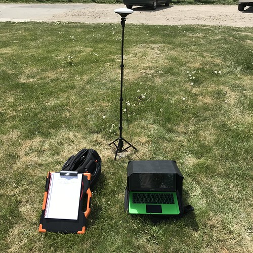
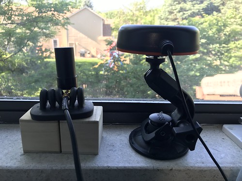
The ability to checkpoint observation files is so useful that I use this mechanism even when I'm not doing a long-term survey. Just yesterday, Mrs. Overclock kindly served as my co-driver as we tested the u-blox NEO-M8U, another GNSS module which includes an Inertial Measurement Unit (IMU). The tiny board-mounted module's IMU contains a gyroscope and accelerometers implemented as a Micro-ElectroMechanical System (MEMS). This can be used to approximate the module's location even when the satellite signals cannot be received - like when we drove through a series of highway tunnels on route US6 west of where we live near Denver Colorado.

I wrote a script that combined gpstool using the Diminuto observation capability, with the peruse script, and another script, hups, that sends gpstool a SIGHUP signal any time any key was pressed on the laptop running my software. This made it easy for Mrs. Overclock to capture the real-time gpstool display in a series of timestamped files, for example as we entered a short tunnel about 215 meters in length, and moments later when we exited it.

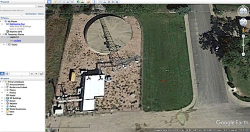
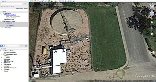
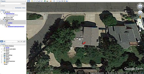
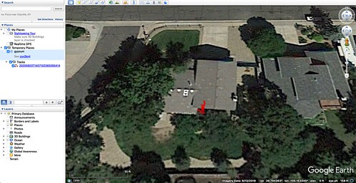
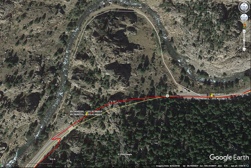
Here's a visualization from Google Earth, produced using the Positioning, Navigation, and Timing (PNT) data captured by gpstool about once per second, converted into a Keyhole Markup Language (KML) file by another Hazer script, then imported into Google Earth. (The red continuous visualized path is not a product of the observation and checkpointing mechanism; but that mechanism was used to identify the locations marked by Google Earth with the yellow push-pins.)

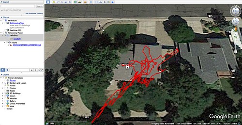
The IMU tracked our path from east (right) to west (left) as we went through the tunnel. (You can see remains of the old pre-tunnel road in the satellite imagery too.) As we left the tunnel and the GNSS signals were re-acquired, the NEO-M8U determined that the IMU had our location a little off and corrected it.

I assure you that we didn't do two sudden tire-smoking turns as we exited the tunnel. Although had we done so, my Subaru WRX would have been the vehicle in which to do it.

Location, Location, Location

That's the punch line for the old joke: "What's the three most important factors in determining the desirability of a piece of real estate?" It's also the answer to "What's the three most important factors that affect precision and accuracy when using Global Navigation Satellite Systems?" It turns out that antenna placement is critical, with antenna selection running a distant second.

The data I'm going to present are not the results of careful controlled experiments. They are derived from datasets I already had lying around that I collected while testing Tumbleweed, my Differential GNSS project. But the data exposes what really matters. Some of this data has already appeared in my prior article Negative Results Are Still Results. In Dilution of Precision I explain how a poor view of the sky both limits the number of satellites your receiver's algorithm can use in its iterative solution, and its flexibility in choosing amongst those satellites to find the ones with the widest orbital separation.  More is better.

For all of these examples, I'll be using two metrics: the diameter of the smallest circle that can drawn around all of the positioning solutions gathered over time (using my tools csvlimits and geodesic), and a visualization of the positioning solutions achieved by converting the CSV output of my software into a Keyhole Markup Language (KML) file and imported it into Google Earth (using my tool csv2kml).

(2020-06-03: This article has been edited to append an additional example at the end.)

Location: NGS KK1446



This used a survey-grade multi-band GNSS antenna (the white saucer-shaped object on top of the tripod) purchased from Ardusimple with the u-blox ZED-F9P GNSS module with my software running on a Raspberry Pi 3B+. The site was an open field containing NGS survey marker KK1446. The view of the sky was excellent. This combination allowed the receiver to use as many as twenty-nine satellites from four different constellations for its solution.

Uncorrected: 0.6925 meters



Corrected: 0.0423 meters



The combination of a survey-grade multi-band antenna with the nearly perfect view of the sky gives an excellent showing. The use of differential corrections reduces the diameter of the solution circle from about 0.7 meters to just about four and a quarter centimeters, a factor of more than sixteen improvement. The corrected view from Google Earth has red marks so small that you need to click on the image to see it in the larger version.

Location: Second Story Window



This used a multi-band GNSS antenna (far left) purchased from Ardusimple with the u-blox ZED-F9P GNSS module with my software running on a Raspberry Pi 3B+. The antenna no longer appears in their catalog, and has no markings on it; but from its weight and dimensions, I believe it has a built-in ground plane (a good thing). The site is a south-facing second-story window in my home office. The view of the sky is fair: only the southern half of the sky is visible, but that part is mostly unobstructed. Even with this partial view, the receiver was able to see as many as twenty-six satellites from four different constellations.

Uncorrected: 5.1404 meters



Corrected: 2.3099 meters



The use of differential corrections reduces the diameter of the solution circle from about five meters to about two and a quarter meters, a factor of about two. This illustrates how differential correction can only do just so much. The uncorrected diameter is very typical of consumer GNSS receivers with their integral patch antennas and a good view of the sky.

Location: Lab Bench



This used a multi-band GNSS antenna purchased from Ardusimple with the u-blox ZED-F9P GNSS module with my software running on an Intel i7-class system. The antenna - the small black vertical cylinder attached directly to an Ardusimple SimpleRTK2B board in a 3D-printed case - is a helical antenna intended for applications like aerial drones, its principle advantages being its light weight and its relative insensitivity to orientation. In my application, the antenna picked up only two of the four GNSS constellations, GPS and GLONASS, during the test period, despite being advertised to pick up all four. The site is the lab bench that sits on the opposite side of my home office, a little over two meters from the same window as above. The view of the sky is poor. Typically only four or five satellites from the two constellations are visible, for example, three GPS, two GLONASS; had this not been a multi-band antenna, it would not have been able to make a position fix using the minimum of four satellites.

Uncorrected: 37.5433 meters



Corrected: 68.2234 meters



You are not imagining this: the uncorrected test run was better than the corrected test run. (I was so skeptical myself that I triple checked that I hadn't gotten the datasets confused.) Neither were worth writing home about. Some of the data points from on the corrected test blew clean over my home to the lot to the east, and even to the lot east of that. This test setup is adequate for regression testing my software for basic functionality, but in no way yields actually useful positioning except at very coarse granularity.

Location: Second Story Window (added 2020-06-03)



This is a later test in which I took the same helical multi-band GNSS antenna (on the left) and tested it in the same location as and alongside the prior setup (which used the antenna on the right) in the south-facing home office window. As before, it uses the Ardusimple SimpleRTK2B board with the u-blox ZED-F9P module, although in this case the Linux/GNU host running my software was an ancient H-P Mini 110 netbook with an Intel i686-class processor. (The u-blox module does all the heavy lifting; my software merely runs the real-time display and collects the data.)

Uncorrected: 3.4650 meters



Merely moving the helical antenna a couple of meters or so from the lab bench to the window makes a huge difference. In fact, in this one instance the small light helical antenna slightly outperformed the larger antenna from the prior test. Moving the antenna to a better view of the sky also allowed it to use as many as twenty-five satellites from all four constellations, versus the barely minimally adequate five satellites from two constellations. The solution diameter of 3.465 meters - over eleven feet - still illustrates how coarse the resolution of uncorrected GNSS is. An aerial drone using this configuration and seeing this kind of resolution would find autonomous navigation problematic.

Location, Location, Location

Differential GNSS can make a big difference, and antenna selection is important. But unless you have proper antenna placement, neither a good antenna nor differential corrections are going to save you.