Showing posts with label Embedded Systems. Show all posts

Wednesday, September 03, 2025

Real-Time versus Real Time

Interesting article from IEEE Spectrum: "How AI’s Sense of Time Will Differ From Ours" [Popovski, 2026-08-13].

Human cognition integrates events from different senses - especially seeing and hearing - using a temporal window of integration (TWI). Among other things, it's the ability that lets us see continuous motion with synchronized sound in old school films at 24 frames per second. But under the hood, everything is asynchronous with different sensing and processing latencies. Which is why we don't automatically integrate seeing distant lightning strikes with the thunderclap, even though intellectually we may know they're the same event.

Machines have to deal with this as well, especially AI in applications like self-driving vehicles. It's non-trivial. "Computers put timestamps, nature does not" as the author remarks. Anyone that develops real-time software - or has spent time analyzing log files - has already had to think about this. I talked about this issue in a prior blog article: "Frames of Reference".

I've also pointed out in a prior article, "Frames of Reference III", that our human sense of simultaneity continuously gives us a false view of reality. If I look towards the back of my kitchen, I see the breakfast table and chairs a few feet away. Since light travels about a foot per nanosecond, I'm actually seeing events that occurred a few nanoseconds ago (plus the communication and processing latency inside me). The back yard that I can see through the window: a few tens of nanoseconds ago. The house across the street: a hundred nanoseconds ago. The mountains to the west: microseconds ago. If I can see the moon on a clear evening: over a second ago. I see all of these things as existing in the same instant of time, but nothing could be further from the truth; my perception is at best an ensemble of many instants in the past, and the present is just an illusion.

AI perception of the real-world will have similar complications.

Wednesday, March 20, 2024

Converting GPIO from the legacy sysfs ABI to the ioctl ABI in Diminuto and Hazer

It could be that no one but me is using my "Hazer" GNSS library and toolkit, or the "Diminuto" C-based systems programming library on which it depends. But just in case: I'm close to finishing testing of the develop branch of both repos, both of which have some major changes to how General Purpose Input/Output (GPIO) - the generic term for controlling digital input and output pins in software - and merging develop back into the master branch.

This was all motivated by my being one of the lucky few to get a backordered Raspberry Pi 5, and putting the latest version of Raspberry Pi OS, based on Debian "bookworm" and Linux 6.1, on it, only to find when unit and functional testing my code that the deprecated sysfs-based GPIO ABI no long worked. This wasn't a big surprise - I had read at least two years ago that the old ABI was being phased out in favor of a new ioctl-based ABI. My code makes heavy use of GPIO for a lot of my stuff, e.g. interrupts from real-time sensors, the One Pulse Per Second (1PPS) signal from GNSS receivers, status LEDS, etc. So it was finally time to bite the bullet and replace all the places where I used the sysfs-based Diminuto Pin feature (diminuto_pin) with a new ABI using the ioctl. Hence, the Diminuto Line (borrowing a term from the new ABI) feature (diminuto_line).

Line is now used in place of Pin in all of the Diminuto functional tests that run on  hardware test fixtures I wired up many years ago just for this purpose, and all the functional tests work. The Hazer gpstool utility has similarly been converted to using Line instead of Pin and has been tested with an Ardusimple board using a u-blox UBX-NEO-F10T GNSS receiver.

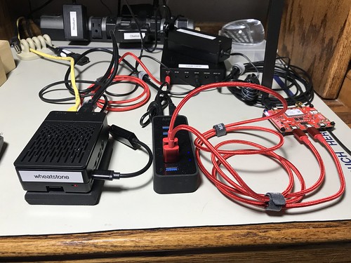
IMG_5717

(That's a Pi4 on the left connected to my test fixture, and a Pi5 on the right connected to the GNSS receiver.)

Two complaints.

[1] The new ABI is woefully under documented. However, I found some code examples in the Linux kernel source repo under tools/gpio that were essential to my understanding. (I chose not to use the new-ish libgpiod for my work, for reasons, but that is a story for another time. I have no reason to believe that it's not perfectly fine to use.)

[2] The way the ioctl GPIO driver is implemented on older versus newer Raspberry Pi OS versions makes it difficult - I am tempted to say impossible, but maybe I'm just not that smart - to write code that easily runs on either platform using the new ABI. Specifically, the GPIO device drivers in the OSes use a different symbolic naming scheme, making it impossible for application code to select the correct GPIO device and line offset portably on the two platforms. But maybe I'm just missing something. (I hope so.)

I like the new ioctl ABI, and expect to use it exclusively moving forward, even though this will orphan Pis I have that might run older versions of the OS. (I think I have at least one example of every Pi version ever sitting around the Palatial Overclock Estate. Ten of them run 24x7 in roles such as a web server, an Open Street Map server, a Differential GNSS base station, and an NTP server with a cesium atomic clock for holdover.) I have tagged the last version of both repos that still use the sysfs ABI.

That's it.

Update (2024-03-23)

I merged the develop branch in to the master branch this morning. Both the Diminuto build and the Hazer build passed sanity and functional testing (and I'm currently running the long-running "geologic" unit test suite against Diminuto). I had tagged the old master branch in both repos with the name sysfsgpio in case I needed to build them, but I don't anticipate any further development of the old code.

Thursday, January 11, 2024

The Disastrous Cultural Evolution of Boeing

The news is full of the most recent Boeing debacle involving the 737 MAX 9 airliner and its door plug that bailed out during flight to land in someone's back yard, leading to sudden cabin depressurization and an emergency landing.

A colleague of mine (Thanks, Jeff!) passed along this interesting and short-ish article on some of the recent history of Boeing, published in The Atlantic about the time of the 737 MAX 8 crashes in 2019 involving the aircraft's Maneuvering Characteristics Augmentation System (MCAS).

Jerry Useem, "The Long Forgotten Flight That Sent Boeing Off Course", The Atlantic, 2019-11-20

The gist:

In 1997, Seattle-based Boeing merges with the much smaller McDonnell Douglas (MCD) in a stock swap. Analysts at the time described it as MCD buying Boeing with the larger company's own money. Surprisingly, the finance-centric (read: MBAs) management of MCD takes over the upper management tiers of Boeing that was previously manned by former engineers. Then, in 2001, the new MCD-based upper management gets tired, apparently, of being questioned by the engineers about cost-cutting and safety concerns, so the entire upper management team moves to new digs in Chicago, 1500 miles away from where the aircraft are built.

WTF?

My favorite jobs over the past four decades plus change have been those in which software, firmware, and hardware product development were closely associated - both culturally and geographically - not just with each other, but also with testing, management, production, and customer support.

My interest in this isn't just from a general product development perspective.

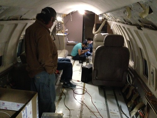
I've had the privilege of having worked on several embedded systems products for the business aviation market, products that could use the term cloud computing in a literal sense. None of those products were flight safety critical. For you aviation geeks, our processes conformed to AS9100, a quality standard, and with DO-178C DAL D, a safety standard, and were tested under DO-160. I even did some hacking with ARINC 429 (an aviation packet bus) and ARINC 717 (an aviation synchronous bus used to log to the aircraft flight data recorder). I got to make the Asterisk open source PBX work with the cockpit two-wire headsets, and with the Inmarsat and Iridium satellite constellations. That job had me crawling around in the equipment bay of a two-engine business jet, and taking short test flights.

(I took these photographs of our Bombardier Challenger 600 test aircraft at Centennial Airport (KAPA) near Denver Colorado.)

On Its Way

Interior Looking Aft

I even got to do some product integration at the Gulfstream Aerospace plant in Savannah Georgia, where I may have walked through Oprah Winfrey's new private jet on the assembly line.

It doesn't get much better than that.

Although our business aviation products were certified for DO-178C Design Assurance Level D - the least safety critical level for which the U.S. Federal Aviation Administration requires certification - we had to have our software certified by an FAA Designated Engineering Representative (DER), essentially an FAA licensed contracted inspector. That turned out to be no small thing. From what I've read, the processes for DAL A - flight safety critical - aviation products were like software development processes dialed up past eleven. The amount of scrutiny and testing that every single line of code receives makes you wonder how the MCAS debacle ever happened. Although it's interesting to note that, like many large aviation companies, Boeing had its own DERs on their payroll.

The cautionary tale of the disastrous cultural evolution of Boeing is a remarkable one, from both a safety and a product development point of view.

Friday, January 05, 2024

Right to Repair, Polish Train Hackers, and the NSA's Ghidra

Google "Polish train hackers" and you'll find dozens of articles in the tech press about this story. Here is the link to the one I read, which was translated from the original Polish. It's terrific. Compelling reading if you're interested in the misuse of Digital Rights Management or the Right To Repair movement. Or if you're into embedded systems development and troubleshooting. Or just if you're into stories of heroic efforts by engineers.


Polish embedded systems hackers use (get this) the U.S. National Security Agency's open source Ghidra tool, originally intended to reverse engineer binaries of computer viruses and other malware, to figure out why high-tech passenger trains, like in the video above, quit working after undergoing routine maintenance - following the train manufacturer's own two thousand page maintenance manual - by a third-party.

What did they discover in various versions of the train software/firmware?

  • Odometer checks that prevent a train from running after a million miles.
  • Year, month, and day checks that prevent a train from running after a certain date.
  • Geofencing checks (naturally the trains have GNSS receivers) that prevent a train from running if it is within the boundaries of a competitor's maintenance depot.

I've used Ghidra myself, and written about it in my blog. The tool includes not just a disassembler similar to objdump, but also a remarkable decompiler that can translate machine code using common C compiler idioms and patterns back into C code. Ghidra understands a wide variety of Instruction Set Architectures. Just recently I've been using it to study the binaries of my own code compiled for a RISC-V target.

DRM and Right To Repair is a big deal in the U.S., Manufacturers of agricultural equipment, like farm tractors costing six figures, have resorted to similar shenanigans to prevent even the farmers who own the equipment from repairing their own stuff. So much so that Right To Repair legislation is coming to the forefront of both state and federal legislators.

Monday, July 03, 2023

Hazer with the U-blox NEO-F10T GNSS Receiver on the Ardusimple SimpleGNSS Board

It's been a while since I talked about my GPS/GNSS efforts. Some time ago I bought a SimpleGNSS board from Ardusimple to try out. The SimpleGNSS has the new U-blox NEO-F10T GNSS receiver. This was my first experience using a new U-blox generation 10 device. It is the first GNSS device of any kind I've used that includes features specific to the latest version 4.11 of the National Marine Electronics Association 0183 standard. And it's the first I've used that's capable of receiving the new L5 band signal from the latest Block III GPS satellites.

I was about ready to dismantle this experiment. But before I removed it from my workbench, I thought I'd update y'all on my latest version of the Hazer library and its gpstool utility.

Hazer is a Linux/GNU/C-based library that supports the processing not only of the usual NMEA 0183 output of GNSS receivers, but also proprietary binary output like UBX from U-blox devices, and CPO output from Garmin devices. It also handles input and output of RTCM messages in support of differential GNSS, yielding geolocation precision down to about a 1.5 centimeters. (I run a DGNSS fixed base and a stationary rover 24x7 at the Palatial Overclock Estate.)

gpstool is the Swiss Army Knife of Hazer. It's one of those old-school tools that has a nightmare of command line options. I use it to functionally test the library, and also as the main component of most of my GNSS efforts. You wouldn't want to use gpstool to navigate cross-country (although I have used it in conjunction with OpenStreetMap to generate a moving map display in real-time). But I find it really useful for testing and evaluating new GNSS devices and just generally futzing around with geolocation and precision timing.

(You may want to click on the short video clips to view them on YouTube instead of from this blog; the UI seems to crop the images, losing some information. You can also click on photographs to see a larger image.)

Here is a short video clip of a Raspberry Pi 4B running gpstool with the NEO-F10T connected via USB.

Besides processing the output of the U-blox device, gpstool is following the 1 Hz One Pulse Per Second (1PPS) digital output signal from the device, which is syntonized to GPS time, and strobes another digital line on the Raspberry PI, syntonized to 1PPS (subject to software latency), to which I've attached a red LED.

Here is a short screen capture that shows the output from gpstool. I've SSHed into the Raspberry Pi from my Mac desktop to run gpstool. The utility uses some simple ANSI screen controls to update the display in real-time. I'm viewing standard output directly from gpstool, but the utility also has the ability to run headless in the background as a daemon, and you can view this real-time display remotely at leisure. (This is how I run my DGNSS systems.)

If you have perused the output of gpstool in any of my prior articles, you may notice a new field in the SAT lines showing the frequency band used by the device to receive data from the indicated satellite, e.g. L1 C/A. Some GNSS devices (like this one) may receive data from the same satellite over more than one band. (I confess this "new feature" is a long delayed bug fix because I botched the handling of new fields in version 4.10 of the NMEA 0183 spec. I have no excuse.)

gpstool isn't just a passive monitor. You can use its command line options to send NMEA, UBX, and other message formats to the device to interrogate and configure it. I did this with the NEO-F10T. Here is a screen shot of a snippet of a script similar to the one I used to generate the output shown in this article.  It sends a batch of UBX messages, sequentially, waiting for an acknowledgement for most of them, to configure the device.

Screen Shot 2023-07-06 at 13.28.38

You can find this script in its entirety in the Hazer repository on GitHub.

Finally, in addition to the standard output, gpstool generates log output on standard error, which here I capture in a file. (If you run gpstool headless, log output can also be automatically directed to the system log without any need for a command line option or API call.)

Hazer gpstool Example Log File

In this example, I have the log output level set to INFO (informational) and above; setting it to the DBUG (debug) level and above generates more output than I typically need unless I am actually debugging new code. (The logging system is a feature of Diminuto, my Linux/GNU/C-based systems programming library on which Hazer and gpstool are built; Diminuto has its own ginormous feature set.)

That's a quick update of some of my latest poking around with GNSS. I'm always on the lookout for new (to me, anyway) GNSS devices to play with!

Wednesday, June 07, 2023

Bug Blast from the Past

I found a Day One bug in some unit test code today that I wrote in 2014, nine years ago. What caused the bug to show up now? I had botched where I had put a thread scheduling yield function call relative to a critical section in the unit test. Apparently this is the first time I have ported this multi-threaded C code to a single-core processor - in this instance, a Raspberry Pi Zero

This is remarkable. As someone said when I related this story to them, it's not uncommon to uncover bugs in code being ported from single core to multi-core processors, but the opposite transition happens seldom enough that this kind of event is rare.

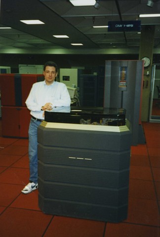
For most of my career - which began before microprocessors even existed - all such computer chips were single core, that is: capable of executing only a single machine instruction at a time. I started writing this library, Diminuto, for a single core ARM4 processor in 2008. But it didn't take long to migrate to inexpensive ARM and Intel chips that could execute more than one instruction at a time. Today, I routinely use small development and test machines that have four or even eight processor cores. As a former colleague of mine, who I met when I worked in Boulder at the National Center for Atmospheric Research and he with Seymour Cray at Cray Computer Company in Colorado Springs, once remarked, your Raspberry Pi 4B single board computer can, by most metrics, outperform Seymour's last supercomputer, the Cray-3 a.k.a. "The Fish Bowl".

The evolution of multi-core microprocessors was largely motivated by, IMNSHO, the end of Moore's Law, at which point doing stuff in parallel was the only way to produce faster microprocessors... faster, at least, for those applications which could take advantage of them. See also: Amdahl's Law.

CRAY-3

Yes, that's a young(er) iteration of me leaning on a Cray-3 in NCAR's computer room at their Mesa Laboratory in Boulder Colorado. Compared to what we can do with computers today, those were the old days, but not necessarily the good old days.

Friday, August 19, 2022

Playing with a RISC-V SBC running Linux

Recently I began playing with a VisionFive RISC-V-based Single Board Computer (SBC). It was designed by StarFive. I purchased it from ameriDroid.

StarFive VisionFive 2-core RISC-V SBC "boron"

RISC-V ("risk five") is a relatively new Instruction Set Architecture (ISA), developed by a team at UC Berkeley, that is entirely open source, unlike Intel and ARM processor ISAs. This is the first RISC-V board I know of that is designed to run Linux (in this case, based on the Fedora distribution). It has two 64-bit 1GHz SiFive U74 CPU cores and eight gigabytes of RAM.

"boron" is my code name for this project. (Every project gets a code name.) I added the nylon feet to hold the board up off the anti-static mat on my workbench. I started out with a keyboard, mouse, and HDMI display attached to the board, but since it supported SSH right out of the box, I quickly reverted to using the command line to build and test my SW, my preferred approach. Also, it reduces the cable clutter on my workbench, which is supporting another project at the moment.

The two projects of mine that I use the most, Diminuto (a C systems-programming library) and Hazer (a GNSS toolkit), were unusually easy to clone, build, and run; unlike most other Linux distros, I didn't have to install any optional packages (much to my surprise). I have successfully completed running all the unit tests for both projects, and am now moving on to functional testing and practical use.

Since my work tends not to be very CPU intensive, I haven't run any performance tests. I'll probably leave that to someone else. I was more worried about SW functionality. But note that this board is more expensive, and and its processor slower, than the ARM-based Raspberry Pi 4 SBCs I use these days.

But the ARM processor design, and the BroadCom implementation of it, on the Pi is closed, and I appreciated the chance to try my stuff out on the open RISC-V, after having read so much about it over the past few years.

Update: 2022-08-20

Just to provide some evidence that I have non-trivial stuff running on the VisionFive, here's a screen snapshot of gpstool running on the board.

Screen Shot 2022-08-19 at 16.22.19

gpstool is the Swiss Army knife of the Hazer toolkit, which is built on top of Diminuto. Here, it's processing input in real-time from a GlobalSat BU-353W10 GNSS receiver. The receiver, a USB dongle, is based on the widely used U-blox UBX-M8030 module.

Update (2023-03-06)

I participated in crowd funding the StarFive VisionFive 2 SBC, which has four 1.5GHz RISC-V processor cores and 8GB of memory.

Calcium

I got the board a few weeks ago and just recently got around to booting up the Debian-based Linux image provided by StarFive. Next step is to get my own software working on it.

Thursday, August 04, 2022

It's About Time

Disclaimer: I am but a humble software/firmware developer. I can barely do basic soldering. But my projects often require that I step out of my comfort zone and come to at least a dilettante's understanding of what is going in the bare metal of the embedded and real-time systems I help develop. In this article, I have left my comfort zone so far behind that I can only see it dimly in the distance, as it waves to me from the horizon.

How do you test the accuracy (correctness) and precision (repeatability) of a clock? By comparing it to another clock. Presumably a more accurate and precise clock. How do you know your reference clock is more accurate and precise? 

Studying this problem is how I learned the term clock trip. This is when you, for example, run a cesium atomic clock on batteries, synchronize (match the clock time) and syntonize (match the frequency) it with a reference clock, take the portable atomic clock on a long airplane flight, and then compare it with the clock under test.

Or, at least, that is how it used to be done. These days, everyone compares their clocks with GPS time, which anyone with a GPS receiver can access. When you synchronize and syntonize a clock with a GPS receiver, it is said to be GPS-disciplined. Then, how good your clock is depends in part on how good your GPS receiver is, how good its own internal clock is, and how good the atomic clocks are in the GPS satellite constellation. But at least you save on plane fare.

I'm not new to the idea of characterizing one clock with another clock.

Timegrapher 

(Click on any image to see a larger version.)
Untitled

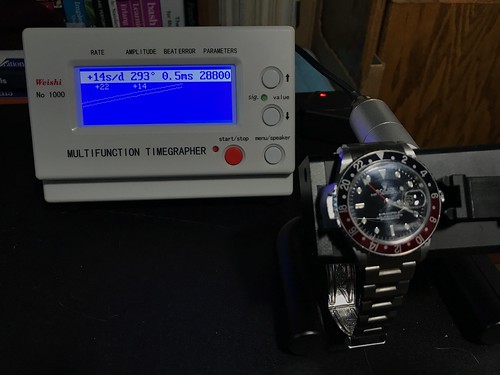
Here is a tool I have used to test mechanical watches: the Timegrapher. It has a sound transducer (a fancy name for a type of microphone) that listens to the ticking of a mechanical watch placed in its test fixture, compares it to its internal quartz oscillator, and displays the results.

I don't find any information about the quartz oscillator used in the my Timegrapher in its documentation. This is a common refrain when testing clocks. But any quartz oscillator - including the one in your quartz wristwatch, if you care to wear one - is likely to be far far better than the spring-driven mechanical movement in the Rolex GMT Master II shown above, and at a tiny fraction of the cost. The same cannot be said, alas, when comparing a quartz oscillator to a clock that is disciplined - that is, continually steered or adjusted - to a GPS reference.

Network Time Protocol

I currently have six small Network Time Protocol (NTP) servers on the local area network at the Palatial Overclock Estate. Two are commercial devices, and the rest are ones I designed and built myself. All but one are GPS-disciplined; the odd one out has an AM radio receiver it uses to pickup and decode the NIST WWVB time transmission. One of the GPS-disciplined servers I built has a cesium chip-scale atomic clock (CSAC) it uses as a frequency source.

Exactly how does one assess the accuracy and precision of a GPS-disciplined clock - especially one that incorporates a cesium atomic clock, a technology from which is currently derived the literal definition of the second - without having a clock that is even more accurate and precise?

That's the problem I continually face: any test instrument - like a digital oscilloscope - that I am able to afford, even one with an oven-controlled quartz oscillator (OCXO) or a temperature-compensated quartz oscillator (TCXO), either of which is far better than the quartz oscillator in my Timegrapher, is likely to be not nearly as good as the GPS-disciplined clock I built. If I try to measure the jitter (short term variation) or drift (long term variation) in my GPS-disciplined clock, am I measuring the error in the clock, or the error in the instrument?
Cesium NTP Monitoring Tool

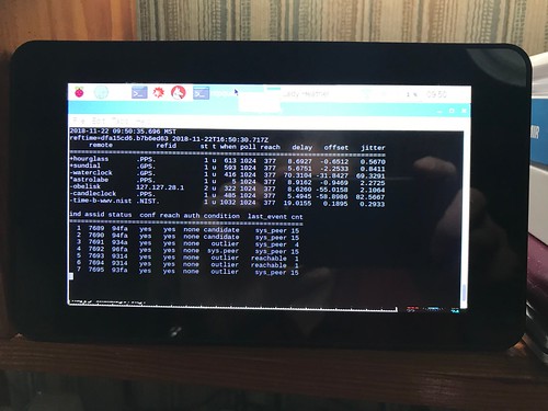
I addressed this problem with my NTP servers by building a little test system, Cesium, using open source NTP software. Cesium runs 24x7, and periodically requests the time from all of my NTP servers plus some public NTP servers on the Internet. The statistical tests in the NTP software score each server. I wrote about this in Monitoring GPS and NTP: Yet Another Raspberry Pi Project

What clock is Cesium using? It's Raspberry Pi has a 19.2MHz crystal oscillator (later Pi models use a 54MHz crystal oscillator). The Raspberry Pi oscillator is not temperature compensated, nor is it GPS-disciplined. And its frequency isn't the final word in how precise or accurate it is. This little tool is useful at a gross level, but it is in no way adequate for more rigorous testing.

UBX-ZED-F9T

This problem came to light again recently when I purchased a Sparkfun board with a U-blox ZED-F9T Global Navigation Satellite System (GNSS) receiver. When its antenna remains in a fixed position over a long period of time (like the window of my home office), so that the long term weighted average of its navigation solution has a low error, the F9T can act as a very accurate and precise time and frequency source. It bases its solution on an ensemble of satellites that are part of the U.S. GPS, Russian GLONASS, Chinese BeiDou, and European Galileo GNSS constellations.

SparkFun: U-blox ZED-F9T

The ZED-F9T is another example of the ninth generation of U-blox GNSS receivers, like the ones I have used in my Differential GNSS (DGNSS) projects that I wrote about in Practical Differential Geolocation. This receiver, though, is especially designed to be a time and frequency source. The SparkFun board is equipped with three SMA connectors: the center one is the input for the receiver's active multiband GNSS antenna, and the other two are outputs for software-configurable digital timing pulses.
Untitled

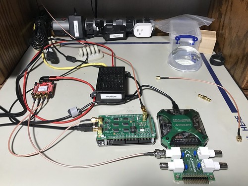
Who doesn't need a GPS-disciplined time and frequency source? I decided to set up test bed using the ZED-F9T - ignoring the fact that I don't have a high-quality laboratory-calibrated oscilloscope (the cost of which could easily run into five or even six figures) - and see what I could see.

The documentation for the F9T say it can emit an output pulse with a frequency up to 25MHz. Although the internals of the F9T are proprietary, this is likely to be a performance limit of its baseband processor, which is probably has some kind of ARM core. The F9T (and in fact all GNSS receivers) has a broadband processor where the digital signal processing of the gigahertz GNSS signals is done, and a more conventional baseband processor where solution computations and input and output messaging is performed. F9T docs say that the device's real time clock (RTC) is driven by a 32KHz crystal oscillator, and suggest that it is not temperature compensated. The F9T's datasheet claims an output time pulse jitter of ±4 nanoseconds. The device is marketed as being suitable for stringent 5G cellular network timing.

 I wrote a script, using my Hazer open source GNSS toolkit, to configure the F9T's first time pulse output to emit a 1Hz pulse, and its second time pulse output to emit a 10MHz pulse. 1Hz, a.k.a. one pulse per second (1PPS), is a commonly used mechanism to syntonize a time clock to GNSS time, while 10MHz is (as we will soon see) a commonly used frequency reference for test and measurement equipment.

Arrayed next to the F9T on my workbench is Rhodium, a Raspberry Pi, and my modest test equipment (described below). The Pi is where my software runs. The Pi has a Universal Serial Bus (USB) connection to the F9T to provide power and a serial connection for configuration and monitoring.

TAPR TICC

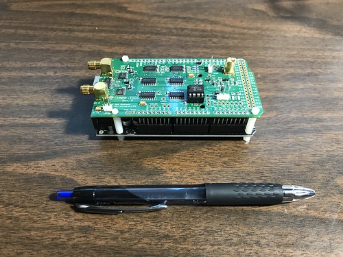
The TAPR TICC is a time interval counter with claimed 60 picosecond resolution. It is produced by the Tucson Amateur Packet Radio (TAPR) organization. It consists of a specialized board mated to an Arduino Mega 2560. It has three SMA connectors: one for its reference clock input (more on that below), and two channels of input that it can timestamp, either in absolute or differential terms. It uses the Arduino USB connection for power, and as a serial connection for configuration and monitoring.
TAPR TICC    

The TICC is a relatively low frequency (albeit high resolution) device, because it outputs a line of ASCII text for every pulse it detects. This makes it suitable for characterizing the 1PPS output of the F9T.

The TAPR TICC documentation has this to say about its timing capabilities.

The TAPR TICC is a two-channel timestamping counter with better than 60 picosecond resolution and less than 100 picosecond typical jitter. It has an Allan Deviation noise floor below 1e-10 for a one second measurement.

The TICC requires an external 10 MHz reference clock at nominally +3 dBm.

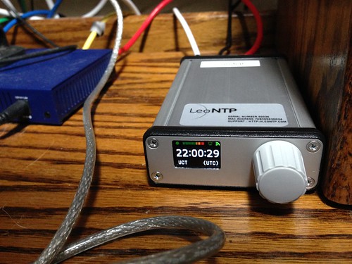
The 10MHz reference clock required by the TICC was provided by a LeoNTP, one of my commercial GPS-disciplined NTP servers, manufactured by Leo Bodnar Electronics. I've had the LeoNTP on my home network for several years. It consistently scores well with my Cesium NTP monitoring tool. I also find its front-panel user interface easy to use. That's two of the reasons I chose it as my reference clock. Another is that it has a BNC connector with a 10MHz output for just this purpose.
Sundial

The docs for the LeoNTP has this to say about its timing accuracy and precision of its BNC time pulse output.

3.3V into High Impedance, 1.5V into 50Ohm PPS/1Mhz/10Mhz Accuracy 30ns RMS, 60ns 99%

While this isn't bad, you'll notice that it's not nearly as good as the claimed performance of the F9T. One of the applications I hope to use the F9T for is as a GPS-disciplined 10MHz reference clock for the TICC and other such devices.

UBX-ZED-F9T-1PPS-metronome-taprticc

This is a screen snapshot of the output of the TICC as it timestamps the 1PPS time pulses from the Z9T. You can see the difference between the time pulses are in generally the range of single digit nanoseconds. Given that its reference clock has a claimed precision that is about an order of magnitude worse than that of the Z9T, this is pretty good, although it's not clear whether I'm really measuring the Z9T, or the LeoNTP.

Digilent Analog Discovery 2

The Diligent Analog Discovery 2 is a recent generation USB oscilloscope. The device claims it can sample analog inputs 100 million times a second (100MS/s). Since the 10MHz (100ns wide) time pulse output of the Z9T generates 10MS/s, I had some hope that this handy tool would serve. (Long time readers will know that this is not my first USB oscilloscope. But it is the first one with this high a sampling rate.)
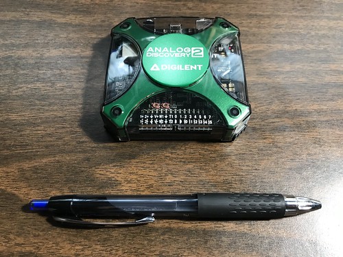
Digilent Analog Discovery 2

All the sampling and measurement hardware is in the little palm-sized pod, which is USB-connected to a host computer (a Lenovo laptop running Windows 10 in my case) for power and to provide the graphical display. The laptop runs Digilent's WaveForms software.
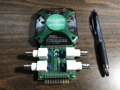
Digilent Analog Discovery 2

One great feature of the AD2 that sets it apart from other USB scopes is that it has an optional adaptor board for BNC connectors. This allows you to use conventional oscilloscope probes with it. Or, in my case, BNC-to-SMA cables.

Hint: if you buy an AD2, regardless of what you use it for, you really want the adaptor board. Depending on your application, you may also want to switch the blue jumper blocks, visible here on the adapter, from the AC pins - as shipped - to the DC pins. Failure to do so causes waveforms like the 1PPS time pulse to look really funky, as the underlying circuitry tries to remove the underlying DC component from the AC signal.

The AD2 documentation has some useful information about the device's clock generator, much of which is over my head.

A precision oscillator (IC31) generates a low jitter, 20 MHz clock.
The ADF4360-9 Clock Generator PLL with Integrated VCO is configured for generating a 200 MHz differential clock for the ADC and a 100 MHz single-ended clock for the DAC.

Analog Devices ADIsimPLL software was used for designing the clock generator. The PLL filter is optimized for constant frequency (low Loop Bandwidth = 50 kHz and Phase Margin = 60°). 

The Phase jitter using a brick wall filter (10.0 kHz to 100 kHz) is 0.04° rms.

The AD2 is capable of being both an oscilloscope and a wave form generator. I'm guessing the former uses the Analog-to-Digital Convertor (ADC), and the latter uses the Digital-to-Analog Convertor (DAC), mentioned above. (The AD2 can also be used as a digital logic analyzer, suitable for commonly used external interfaces on microcontrollers and embedded processors, like SPI, I2C, and UART.)

Low Frequency Events

Pointing the AD2 at the 1PPS time pulse output of the F9T yielded the following wave form.

UBX-ZED-F9T-1PPS-metronome-DC

Once I collected some 1PPS output samples in the AD2, I used the software's built in capability to measure the period between two successive pulses.
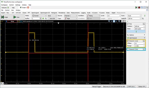
UBX-ZED-F9T-1PPS-measurement-1

The AD2's measurement of the pulses being 1.002 seconds apart (a period equivalent to a frequency of about 9.98MHz) is not great, and not typical of the timing reported by the TICC. Once again, it's not clear I'm measuring the F9T, or the goodness of the AD2. But given the AD2's sampling rate of 100MHz, I would expect a measurement error of as much as ±10ns, once again not as good as the F9T's claimed ±4ns. (You're probably detecting a theme here.)
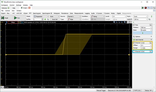
UBX-ZED-F9T-1PPS-blowup-1

Cranking the display resolution up on the stored samples, in effect zooming in on the graph, the WaveForms tool shows what the docs say is a "noise band indicating glitch or higher frequency components than the sampling frequency". (It's not clear to me how the device knows anything about what's going on above its sampling frequency.)

UBX-ZED-F9T-1PPS-blowup-2

Cranking the resolution a little higher shows a graph that indicates the actual points at which the 1PPS wave form was sampled. Now we can see some ground truth (which was probably already obvious to the hardware folks): the display consists of straight lines between successive sampling events. The rise of the 1PPS output line from ground to VDC (the 3.3V logic level of the F9T) cannot be instantaneous, and in fact is captured by the 100MHz sampling rate of the AD2. This explains the slight jog in the leading edge of some of the 1PPS pulses that is visible in the lower resolution displays. (This insight will be even more useful shortly.)

High(er) Frequency Events

Pointing the AD2 at the F9T's 10MHz time pulse output, we would expect see even more measurement artifacts, since the AD2's sampling rate is merely ten times the frequency of the signal we are measuring.
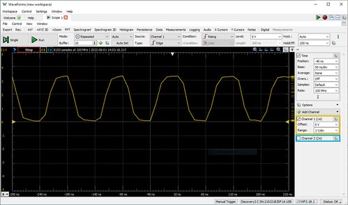
UBX-ZED-F9T-10MHz-metronome-DC

The 10MHz time pulse is a digital signal, but not a sine wave. But its visualization by the AD2, and the fact the output signal cannot change instantaneously, makes it look like one.
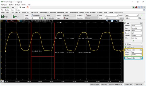
UBX-ZED-F9T-10MHz-measurement-2

Measuring the period of the time pulse becomes even more challenging. At what point do we compare successive pulses? The TAPR TICC, for example, counts anything that rises above a threshold of 1.7V as a pulse. Doing so here gives us a frequency of about 9.83MHz.

UBX-ZED-F9T-10MHz-measurement-3

It occurred to me that measuring at the point in the pulse where it starts to rise might be a better indication of the goodness of the F9T. Doing so gives us a frequency just barely short of 10MHz, off by a claimed 0.2ns, probably within the measurement error of the AD2, and certainly within the claimed precision of the F9T. (0.2ns is smaller than the period of the sampling rate, 10ns, so once again it's not clear to me how the instrument knows this.)
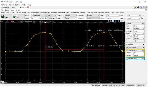
UBX-ZED-F9T-10MHz-measurement-5

Cranking the display resolution a little higher shows us the AD2's sampling points on the 10MHz wave form. (It also shows us why the wave form is a little funky looking, as the straight lines between samples become more obvious.) We can more carefully choose the data points that we used to measure the interval between time pulses.

UBX-ZED-F9T-10MHz-measurement-4

It occurs to me (again, probably obvious to the hardware folks) that how good the 10MHz output of the F9T appears will depend upon both the input impedance - effectively the speed at which the analog signal can change, due to the electrical characteristics of the circuit - and the measurement threshold (e.g. 1.7V?) of the device that is making use of it.

Conclusions

Neither TAPR TICC nor the Digilent Analog Discovery 2 are good (read: expensive) enough to really judge the quality of the output of the U-Blox ZED-F9T. I'll leave that to the folks with the $25,000 (or more) oscilloscopes with the oven-controlled quartz crystals. However, they were absolutely indispensable at debugging my configuration script for the F9T.  Without them, I would have had no idea if I were even in the ball park with the fairly complex messaging my software was sending to the F9T. For no other reason than this, I recommend cost effective instruments like these for any embedded software developer's toolkit.

As for my own applications of the F9T, my opinion is: if it's good enough for 5G, it's probably good enough for me.

Tuesday, January 25, 2022

Fun Facts to Know and Tell: RPi on an SSD, Microsoft Linux

As an aside from my main projects - mostly my GPS and LTE-M efforts - I've been working on a couple of things that I am a little surprised to have worked as well as they have (even though they may not be perfect).

Raspberry Pi Running From An SSD

The latest Raspberry Pi board - the 4B - introduced a firmware-based boot loader than can be easily configured to boot from something other than the resident micro SD card. It was pretty easy to configure it to boot from a USB-attached SSD.

Here's an image of one of my Raspberry Pi 4B SBCs sitting on top of a Samsung T5 that it booted from and is running off of. (The T5s have since been replaced by the newer Samsung T7.)

Untitled

I also found some instructions to enable the SATA TRIM command on the SSD so that the OS could get sectors on the SSD erased as a background activity.

It's not perfect: the SSD pulls enough power that I had to add an externally powered USB hub to run other stuff like GNSS receivers and LTE-M radios. But I'm running a full blown Ubuntu OS instead of Raspberry Pi OS (a.k.a. Raspbian). I run Ubuntu elsewhere on a Raspberry Pi using a micro SD card, but this is a lot more spacious, not to mention a lot faster.

Microsoft's Linux Distribution

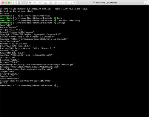
Remarkably, Microsoft has created its own Linux distro for the x86_64 target: the Fedora-ish CBL-Mariner (for Common Base Linux). It's intended as an internal Linux distro for Microsoft's Azure cloud infrastructure. I got it running as a virtual machine under VMware Fusion on my old desktop Mac. It works pretty well; I got my Diminuto C library and my Hazer GPS project running on it with very little effort.

Screen Shot 2022-01-25 at 10.05.16

It's not perfect: weirdly, it can't display the Unicode degree symbol, which is used in a couple of places in my Hazer code (gotta believe this is just a Unicode font issue). And the IPv6 unit tests in Diminuto don't pass 100% (current thinking this has nothing to do with CBL-Meridian, but with a change I made in my company web site). But otherwise I'm processing input as usual from a GNSS USB dongle.

Update 2022-01-25: The degree symbol display was a day-one bug in my Hazer code, related to setting the locale, that didn't manifest under Debian-based OSes. (If I had followed my own documentation, this would not have occurred.) The IPv6 issues were breakage caused by my own changes in the Digital Aggregates web site to support HTTPS and were unrelated to either CBL-Meridian or support in Diminuto for IPv6.

Friday, January 07, 2022

Test What You Detonate, Detonate What You Test

Another great article from the national security blog War On The Rocks: "When Software Bugs Go Nuclear: Testing A Digital Arsenal" by Laura Epifanovskaya, a researcher formerly in the U.S. Department of Energy's nuclear weapons program.

Motivated by the fact that the U.S. nuclear weapons stockpile is transitioning from analog to digital control systems - so as to interface with the digital systems in the latest generation of strategic weapons delivery platforms - she writes about the need for formal methods, Design For Test (a design methodology that applies to software as well as hardware), and NASA's motto "Test what you fly, fly what you test", in critical reliability systems.

There is a lot here that is applicable, not just to nuclear weapons, but to any complex high-technology system that absolutely, positively has to work right the first time - and never work when it's not supposed to. Her article also has some interesting tidbits into how nuclear weapons are tested without actually setting off a fusion reaction. Fascinating stuff.

Tuesday, April 06, 2021

Ghidra 9.2.2

 Ghidra is an open source graphical tool produced by the U.S. National Security Agency (NSA) to analyze binary (compiled) software images for a wide variety of hardware targets and compiler platforms. Amongst its many capabilities are generating a disassembly listing and (remarkably) generating a decompiled listing back into C. This latter case requires that the tool recognize idiomatic instruction sequences produced by common compilers like GNU C, as well as deal with some special cases in which assembler code is inserted inline by the C developer, e.g. for memory barriers, low level synchronization primitives, and accessing special hardware registers.

The NSA released version 9.0 of Ghidra to the public just about two years ago. I wrote a couple of articles (see references below) here about using it to reverse engineer compiled code from my Diminuto, Hazer, and Scattergun projects. I did find a couple of bugs - multiple symbol tables in shared objects confusing the disassembler, and inserted memory barrier instructions confusing the decompiler - reported them, and got useful feedback from one of the developers.

Yesterday I installed the latest public release of Ghidra, 9.2.2, and tried two of the specific cases that were problematic that I wrote about in my two blog articles. Casual perusal of the Ghidra 9.2.2 disassembled and decompiled output for ARM7 binaries suggests both of these issues have been resolved. I updated both articles with remarks to this effect, and included screenshots of the updated output.

Reverse engineering has a lot more applications than just cybersecurity. Analyzing deliberate malware isn't typically my area; but debugging proprietary embedded software, and integrating my and my clients' new code with legacy systems, is an integral part of what I do for a living. Tools like this can be crucial for dealing with undocumented or under documented legacy systems. Reverse engineering tools like Ghidra should be in the toolkits of embedded and other low level systems developers.

References

C. Overclock, "Ghidra", 2019-03-25

C. Overclock, "Decoding Special Machine Instruction Sequences with Ghidra", 2019-03-26

Tuesday, March 23, 2021

Where the RF Meets the Road

My Hazer project (com-diag-hazer) - the basis for all my GPS/GNSS work that I've written about - depends mightily on my Diminuto project (com-diag-diminuto) - my C systems programming library and framework - for its infrastructure. Testing some of the Hazer features finally got complicated enough that I built a dedicated test fixture for that project, just as I had to build a little test fixture for  Diminuto that I described in Where the Silicon Means the Road.

Diminuto GPIO/Hazer 1PPS Test Fixture

While Hazer's gpstool utility supports a wide variety of GPS/GNSS receivers, the one I chose for the test fixture is a SparkFun board equipped with a u-blox NEO M9N device. Here is some gpstool output generated while exercising the M9N.

Hazer gpstool using a u-blox M8N

I chose the M9N because it can receive and process transmissions from the satellite constellations of the U.S. GPS (a.k.a. NAVSTAR) system, the Russian GLONASS system, the European Galileo system, and the Chinese BeiDou 2 (a.k.a. COMPASS) system simultaneously. This tests more code paths in the underlying Hazer library and in gpstool.

Diminuto GPIO/Hazer 1PPS Test Fixture

The M9N is powered by a USB C connection to a dedicated Raspberry Pi 4B running Raspberry Pi OS, the Debian-based version of GNU/Linux formerly known as Raspbian. The USB connection is also the serial communications channel between the Pi and the M9N. The Pi runs headless; when necessary, I ssh into it from my desktop Mac and use the command line interface (although in a pinch, I have connected up a display, keyboard, and mouse to the Pi, or even attached a USB-to-serial adapter to its console port pins).

Diminuto GPIO/Hazer 1PPS Test Fixture

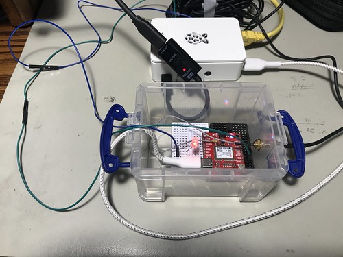
You can see the SMA Radio Frequency (RF) connector emerging from the container, where it connects to the coaxial cable of the GNSS antenna used by the M9N. The small multi-band active patch antenna sits on the top shelf of my workbench within view of the window.

u-blox Multi-band Active GNSS Antenna

You can also see a green wire and a blue wire that run from the M9N container to the Raspberry Pi.

The green wire connects the 1PPS ("one pulse per second") signal from the M9N to a General Purpose Input/Output (GPIO) pin on the Raspberry Pi. 1PPS is a standard precision timing signal derived from the GNSS solution by the receiver (although not all of them export it, and when they do, the mechanism varies). I make use of 1PPS in all of my GNSS-disciplined Network Time Protocol (NTP) micro servers that I've written about previously, including the one that incorporates a chip-scale cesium atomic clock. When gpstool is configured to monitor the 1PPS signal, it uses Diminuto's GPIO feature to interrogate the input GPIO pin using the select(2) system call inside a dedicated POSIX thread (which is also a Diminuto feature).

The blue wire connects an second, output, GPIO pin on the Raspberry Pi to an LED in the little container where the M9N is mounted. When gpstool monitors 1PPS, it can be configured for the thread to strobe the second GPIO pin to follow the 1PPS signal. This is not just a test of Hazer and gpstool, but a test of Diminuto's GPIO feature as well.

Diminuto GPIO/Hazer 1PPS Test Fixture

My hardware engineer colleagues will confirm that I'm not a hardware guy by any stretch of the imagination. But hacking together these little hardware test fixtures gives me peace of mind. As long as I see that LED blinking at 1Hz, I know that, while my code is not perfect, it is at least sane.

Thursday, March 04, 2021

The OpenStreetMap Moving Map on Mobile Devices

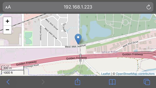
One of the advantages of implementing tools as web applications is that it opens the possibility of running them on a wide variety of platforms, with browsers that support JavaScript and HTML5, with little or no additional effort. I'm a little embarrassed to admit that it just recently occurred to me that I should be able to run my OpenStreetMap (OSM) Moving Map web app on my iPad and iPhone. So I did. It worked fine.

Here is a screen snapshot from my iPad using Safari.

Untitled

Here is one from my iPhone 7, also using Safari.

Untitled

And for good measure, here is a screenshot from my Google Pixel 4 development phone using Chrome under Android 11. It worked fine too.

2021-03-04_12-44-59

I routinely run the web app on Safari, Firefox, and Chrome on my desktop Mac or my Mac laptop, and on Firefox and Chrome on an x86_64 Linux server. Now I can add genuine mobile devices to that list.

But wait! There's more!

I described in prior articles about this project, code-named Tesoro, how the server-side JavaScript program channel.js serves as a conduit between my Hazer C-based GPS software in the field, which forwards geolocation data in JSON over UDP, and my web application whose OSM-based moving map is steered by that incoming data stream. Alas, channel.js only services a single data source at a time (although you can run several instances simultaneously using different UDP port numbers).

Tesoro now includes another server-side JavaScript program, controller.js, that can handle an arbitrary number of geolocation data sources concurrently, all using the same UDP port number, and provide an individual URL for each one for the Tesoro web application. I have an instance of controller.js executing now on one of the Raspberry Pis that runs 24x7 at the Palatial Overclock Estate, serving as the sink for any geolocation project in the field (or for a playback of the dataset collected from any such project), and as the source of that same data for any moving map displays on my internal network.

Wednesday, February 24, 2021

The OpenStreetMap Moving Map In Real-Time

The moving map display I demonstrated in the forty-five minute video in A Moving Map Display Using OpenStreetMap (2021) was the result of playing back a dataset I had collected in 2020 during a test of a u-blox UBX-NEO-M8U, a relatively complex piece of kit that included not only a Global Navigation Satellite System (GNSS) receiver but also an integrated Inertial Measurement Unit (IMU). I wanted to capture a moving map video in real-time just to remind myself that it could be done, so this morning I did just that.

The Overview

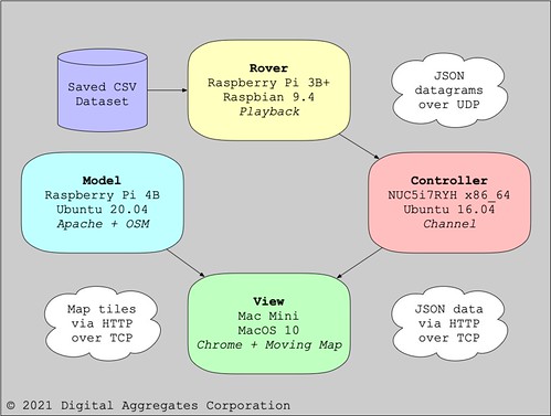
You might recall from that prior article, my implementation consists of four components.

The Rover is either a GNSS receiver connected to a computer running my Hazer gpstool software to collect geolocation data in real-time, or a computer playing back such a dataset.

The Model is an OpenStreetMap (OSM) tile server that serves up graphical map segments and associated metadata via HTTP requests over TCP.

The View is your favorite modern web browser supporting JavaScript and HTML5 that renders the moving map using tiles fetched from the Model as it is steered by the Controller.

The Controller is a conduit that captures the datagrams of JSON data transmitted by the Rover over UDP and makes them available to the rest of the system via HTTP requests over TCP.

Tesoro2

The Model, View, and Controller are all part my Tesoro project.

The Good Stuff

We'll start off with today's fifteen minute (14:49) video, captured on a display at my home base while I drove my Subaru WRX equipped with the Rover around the neighborhood. Feel free to skip around. (If the video doesn't show up for you, you can find it on YouTube. For best results, open the video up in a larger window, and select the High Definition version.)

The Test Setup

The Model was the same Raspberry Pi as before, running the OSM software stack as an Apache web application.

The View was my desktop Mac Mini with a Cinema Display, using QuickTime to capture the video from the Safari web browser running the Tesoro client-side movingmap JavaScript program.

The Controller was the Tesoro channel server-side JavaScript program running under Node.js on another Raspberry Pi. It is the same RPi I use as a Real-Time Kinematic (RTK) corrections server for Differential GNSS (DGNSS) for my Tumbleweed project.

The Rover consisted of a relatively inexpensive USB-connected receiver, a GlobalSat BU-353S4-5Hz, based on a SiRF Star IV chipset. (SiRF is a division of mobile phone chip maker Qualcomm). It was connected to a GPD MicroPC running Hazer's gpstool under Ubuntu MATE. The tiny palmtop computer was equipped with an external NovAtel MiFi USB730L LTE modem that it used to transmit its JSON datagrams containing geolocation data back to home base.

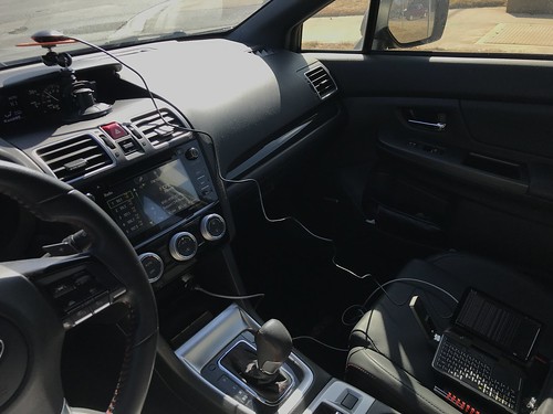
Here is the Rover sitting in the WRX during the test; the GPS receiver is at the far left on a mount on the dashboard, and the PC is sitting on the passenger seat at the far right with the LTE modem visible on its left side.

IMG_4364

Here's a close up of the BU-353S4-5Hz receiver in my lab. The little USB dongle is not much larger than a wristwatch face, and includes the GPS receiver, the active (amplified) patch antenna, and the USB interface which provides both connectivity and power. It's magnetically mounted on a steel plate that serves as a ground plane, a reflective surface for GPS radio waves.

USGlobalSat BU-353S4 GPS Receiver with USB Interface

The GPD MicroPC, shown below on my lap bench with the LTE modem attached on its left side, is basically a pocket-sized ruggedized industrial PC. Although I don't do any touch typing on its chicklet keyboard, I really like the fact that the little Intel Celeron-equipped palmtop incorporates a lot of useful interfaces, including WiFi, an RJ45 Ethernet jack, and an RS232 serial port with a DB9 connector.

GPD MicroPC running Ubuntu MATE

UDP vs. TCP

If you watch the video, and pay attention to the JavaScript console at the bottom, you will notice that the movingmap script occasionally reports missing JSON datagrams. This is typical of my experience in the field using LTE modems and the best effort User Datagram Protocol (UDP) to transmit geolocation updates to the home base. This causes the moving map display to briefly stall and then jump forward as it catches up to the real-time data.

As you might expect, using the guaranteed delivery Transmission Control Protocol (TCP) instead of UDP solves this problem. And indeed, my initial implementation years ago used TCP. But what I found during these kinds of real-time visualizations, especially in locations with spotty cellular reception, is that the display could lag many seconds behind real-time as the TCP/IP stack retransmitted lost packets. And once behind, it never caught up. In fact, it sometimes got progressively worse. It was far better to have the map pointer jump forward than to permanently and increasingly lag behind what was happening in meat-space.

I talked about this at length in Better Never Than Late (2017): in this particular real-time application, it is better to lose packets, or drop packets that arrive out of order, than it is to wait for the network stack to ensure perfect reliability. Besides, my Hazer software saves all the geolocation information on the Rover as a dataset of Comma Separated Values (CSV). So at worst, you can play back the dataset with perfect fidelity when the Rover returns to home base.

(Note: edited several times for corrections and clarity.)

Friday, February 19, 2021

A Moving Map Display Using OpenStreetMap

Google Maps is a treasure. Hardly a day goes by that I don't use it. If I see a news item that interests me that includes an address, or even just a neighborhood, chances are good I'll be looking it up. By the time Mrs. Overclock and I got to Helsinki Finland to attend the World Science Fiction Convention in 2017, I had already "walked" all around the neighborhood of our hotel using Street View.

But although using Google Maps this way for me is free, it is a costly commercial product to develop and support. The maps have to be continuously updated with corrections and changes. The Street View images are routinely laboriously updated and ground truth established by humans driving extensively instrumented vehicles. The Satellite View images are updated frequently enough that I am often surprised to find that the season or the landscaping has changed since the last time I looked at my own neighborhood. It can't be cheap. Google supports this "free" service through a combination of fees for businesses that choose to advertise on this platform, and by licensing its use for products that use this platform for their own mapping needs.

By now, anyone reading my blog has come to realize that I have had a long running, broad, and deep, personal effort at writing applications using the U.S. Global Positioning System (GPS), and more broadly, other Global Navigation Satellite Systems (GNSS). More recently I branched out to include Inertial Measurement Units (IMU). This is part of my Hazer project, the source code repository for which can be found on GitHub. I am understandably interested in mapping the results of my tests, either in real-time or as part of my post-test analysis. Google Maps would have been ideal for this, but the price tag was a little high for something that amounts to an intensive hobby.

In my article Better Never Than Late (2017), I tracked a mobile GPS unit in my car by transmitting its geolocation data back to my home office via an LTE modem, to be mapped in real-time using Google Earth, an application program that provides a programmatic way to use satellite imagery. This worked great; but sometime between 2017 and 2018 the capability to do this in real-time with Google Earth stopped working. I was still able to do the post-test mapping by importing the data into Google Earth in Keyhole Markup Language (KML) form, as illustrated in my article Dead Reckoning (2020). But I wanted a solution for a real-time moving map display.

Recently I became aware of OpenStreetMap (OSM), an open-data, community-driven, project to provide an alternative to Google Maps for exactly the kind of real-time mapping in which I was interested. Thus was born another project, Tesoro, also hosted on GitHub, with the goal of incorporating OSM with Hazer to create a real-time moving map display.

Demonstration

Before I get to the nuts and bolts of Tesoro and OSM, let's go right to the good stuff: a video of the moving map display that I implemented. This is a forty-five minute (45:47) video, so no one (not even me) is going to want to watch all of it. But it's fun to skip around and watch different parts. For best results, watch this video in a separate YouTube window, and if your user interface supports it (not all do), choose the High Definition option so you can read the labels on the map. Opening it up into Full Screen mode helps too. Or be prepared to do a lot of squinting. (If the video below doesn't show up for you, try this link to the video on YouTube.)


This test used a playback of geolocation data I collected during IMU testing conducted on 2020-09-17. The playback mechanism uses the same UDP-based networking to feed the Hazer data stream to Tesoro that I have used previously in the field, so I would expect it to work almost as well with a real-time feed, subject to the occasional data loss I witnessed using LTE modems. (In Better Never Than Late I make the case as to why UDP, and not TCP, is the correct internet protocol to use for this. Alas, an efficient and easy to use method of encrypting and authenticating UDP traffic - while maintaining the characteristics of UDP that I find important - is in my opinion an unsolved problem.)

Overview

Tesoro broadly consists of four components: the Rover, the Model, the View, and the Controller. Web developers will recognize the Model-View-Controller (MVC) nomenclature used to describe a design pattern for interactive applications. GNSS developers will recognize Rover as the mobile portion of a Differential GNSS (DGNSS) system. (As always, you can click on any image to see a larger version.)

Tesoro

Although most of my development of Tesoro was done by running all of these components on a single computer, that didn't reflect how I expect the system to be used in real life. So for the video above, I split the components onto four different computers.

The Rover

The Rover plays the role of the component in the field, running the Hazer gpstool application and forwarding the resulting geolocation data via UDP back to the home base. For this test, the Rover was one of my Raspberry Pi 3B+ development machines running a version of the Debian Linux distro called Raspberry Pi OS (formerly called Raspbian).

gpstool saves geolocation data in a Comma Separated Value (CSV) format so it can be easily imported into a spreadsheet. The Hazer csvmeter script reads the stored CSV data and meters it out at approximately the same rate - typically 1Hz - as it was originally generated by the GNSS receiver under test. The output of csvmeter is piped to the Hazer csv2dgm utility that trivially converts it into JavaScript Object Notation (JSON) - the standard data serialization format used by JavaScript and lots of other applications because it is far simpler than eXtensible Markup Language (XML) - and sends the resulting datagram on its way.

The Rover can be tested by using the Linux/GNU utility socat to receive the datagrams and display them on the console.

The Model

The Model (short for Data Model) provides the database of map data used by the moving map display. The Model is an OpenStreetMap tile server, a server-side web application and database that provides tiles - graphical map segments - via Hyper Text Transfer Protocol (HTTP). It is hosted on a Raspberry Pi 4B computer with a two terabyte (2TB) Solid State Disk (SSD) in addition to its own root file system on a microSDcard.

Untitled

This tiny Single Board Computer (SBC) runs, not the typical Raspbian, but a full blown version of Ubuntu, another Debian-based Linux distro. I chose Ubuntu over the usual Raspbian that I run on the other ten Raspberry Pis that run 24x7 at the Palatial Overclock Estate because the OSM stack was known to work under Ubuntu. Could it run under Raspbian? Got me. When I found out that there were instructions for installing OSM under Ubuntu 20.04, and there was a version of Ubuntu 20.04 that could be installed on the Raspberry Pi 4B, I looked no further. Installing Ubuntu, then the entire OSM stack, then the map data for North America, then building the map database, on the Raspberry Pi was a relatively simple but time-consuming process.

I was careful to keep the map dataset (which is very large) and the Postgres database (which is very active) on the SSD. Given that just today I saw an ad for a one terabyte (1TB) microSDcard, it might be possible to implement a tile server without the SSD.

The Model can be tested by issuing an appropriate HTTP request from a browser or the Linux/GNU command line utility wget and seeing what comes back.

The Controller

The Controller provides the data stream that steers the moving map. It is implemented by channel, a small server-side JavaScript program I wrote that stands up a microscopic HTTP server. The channel receives the JSON datagrams from the Rover via UDP and caches the most recent one. When channel receives an HTTP request of any kind (it's not picky) over TCP, it responds by replying with the latest JSON datagram.

The channel is merely the conduit through which the JSON datagrams from the Rover can be received by the client-side web browser a.k.a. the View. Non-web developers may be surprised (I was) at how difficult this simple requirement is to solve. Browser security is an ever tightening chain of rules and sandboxing designed to keep malicious web sites from stealing your identity or infecting your laptop with malware. A lot of solutions you might take for granted as being feasible are actually deliberately impossible.

JavaScript programs running on the server-side under the standard Node.js compiler/interpreter have no such restrictions, however. I ran the channel JavaScript program on one of my x86_64 Ubuntu development systems, but any Linux/GNU system running Node.js would do.

The Controller can be tested by running channel and then making a web request using a browser or wget.

The View

The View is the visualization engine of Tesoro. It consists of a lot of client-side JavaScript code running inside of the web browser of your choice, being steered by the JSON it periodically fetches via HTTP from the Controller, and then rendering the appropriate map segments it requests from the Model. The View is implemented by a combination of Hyper Text Markup Language (HTML) files that download and run my movingmap JavaScript program. movingmap is built on top of Leaflet (1.7.1), a widely used JavaScript library that provides a client-side API to OSM. It is Leaflet that does all of the heavy lifting with OSM.

The View client-side HTML and JavaScript code (including Leaflet) are hosted on the Model, the OSM tile server, as just another Apache web site application. They are downloaded and executed inside the web browser on whatever computer the browser is running on. You can probably run the View on any modern web browser that supports JavaScript. The video above was recorded with QuickTime using the Google Chrome browser running on my desktop Apple Mac mini running macOS 10 with an Apple Cinema Display. But I have also run the View with Firefox on an x86_64 Ubuntu system, and with both Firefox and Safari on the same Mac.

Tesoro includes several HTML web pages that can be used to incrementally test the View and the rest of the software stack, first displaying a static map at a fixed location, then a static map whose latitude and longitude are specified as a query in the Uniform Resource Locator (URL), then finally as dynamic moving map display being steered by a user-specified channel.

Details

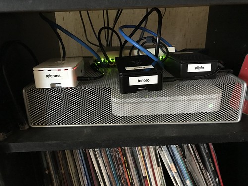
This is an image of the Raspberry Pi that is the OpenStreetMap tile server (center). It resides in an old stereo rack alongside my web server (left), and a Real-Time Kinematic (RTK) update server (right) that is part of my DGNSS project.

IMG_4345

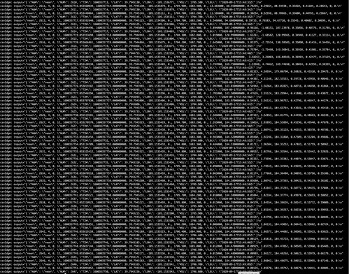
This is the console output of the Rover's csv2dgm utility, which is written in C and is part of Hazer. When debugging output is enabled, csv2dgm displays both the incoming CSV record and the outgoing JSON datagram.

Screen Shot 2021-02-17 at 1.41.37 PM

Although for this example I was playing back a dataset of CSV records previously recorded as part of an actual field test, the same csv2dgm utility is used in the script that runs on the Rover in the field; this output is an easy way to verify that the Rover is generating datagrams before deploying it.

The Controller's channel JavaScript program that runs under Node.js is pretty chatty as well. Every time it receives a datagram over UDP, it displays its JSON payload as well as the sender from which it was received. Every time the View (or anyone else) issues an HTTP request over TCP, the program displays the requestor and the JSON it was sent.

Screen Shot 2021-02-17 at 1.42.52 PM

This output is especially useful since it can be saved as a permanent record on the local computer on which channel runs, independent on to whether the CSV dataset saved on the Rover in the field is eventually recovered.

All three of the web browsers I tested with - Chrome, Firefox, and Safari - have very useful debugging tools built in. In this screen shot from the video above, you can see the moving map on the left, and an optional console log on the right. Tesoro's movingmap client-side JavaScript program makes use of this log to reveal what it is doing. All three browsers have a console log like this, variously called "JavaScript Console", "Web Console", or a "Console" tab on a "Developer Tools" window.

Screen Shot 2021-02-19 at 12.24.55 PM

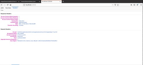
All three browsers also have tools to examine the headers used in the HTTP protocol. This is useful for debugging all three components, Model, View, and Controller, since all use HTTP.

Screen Shot 2021-02-17 at 10.00.57 AM

The README file for the Tesoro repository on GitHub has links to the pages I used to learn how to install Ubuntu on the Raspberry Pi, to install the OSM software stack, to download the map data, and to build the Postgres database, all on the Model tile server.

In addition, the repository includes a text file of mostly unstructured notes that might be useful if you get stuck trying to reproduce my results. Be aware, though, that not all of the notes led to something I actually used or did; some were dead ends.

Conclusions

I'm a little surprised how well this project worked, mostly because I wasn't a web developer when I started it. I'm not a web developer now, either. JavaScript will not be appearing on my LinkedIn profile.

But thanks to having hacked other developer's JavaScript on various paying gigs that had a web component, and to the wealth of documentation I found online, I was able - as usual - to learn from people smarter than myself.

(Note: edited several times for corrections and clarity.)