Negative Results Are Still Results

Tumbleweed is the code name for my experiments with the u-blox ZED-F9P module and its ability to both generate and accept differential corrections to Positioning, Navigation, and Timing (PNT) solutions using Global Navigation Satellite Systems (GNSS) like the U.S. Global Position System (GPS). Tumbleweed leverages and expands the work I did in another project, Hazer, an open source C-based library and toolkit that I wrote to help me explore the world of satellite-based geolocation.

Hazer and Tumbleweed have challenged my capabilities as an embedded software developer. The artifacts that have come out of those projects include a Network Time Protocol (NTP) server with a cesium atomic clock, and a Differential GNSS (DGNSS) system that has the potential to achieve accuracies at the centimeter level or better from a technology - GPS -  that fundamentally is limited to accuracies of about five meters or so. At the beginning of both of these efforts I pondered how I was going to test them. Projects which, if they were successful, would result in devices that could measure time and space to a resolution far better than any measurement instrument I owned, could afford, or could borrow.

In this longish article I will try to describe the difficulties in testing the DGNSS system that came out of Tumbleweed, and how I tried - with varying amounts of success - to address them.

You can click on any image to see a larger version. A list of references and sources for this work can be found in the README file in the Hazer repository on GitHub.

Precision versus Accuracy

There are two basic and different aspects to measuring systems like Tumbleweed: precision and accuracy. The classic way in which the difference between precision and accuracy is explained is this:

An archer shoots arrows at a target. If an arrow lands right in the bullseye, the archer is said to be accurate. If all of the arrows land near the same spot on the target (but not necessarily in the bullseye), the archer is said to be precise. Accuracy is about correctness. Precision is about consistency. The archer wants to be both accurate and precise.

You can see how this applies to devices like clocks. A precise clock strikes noon at the exact same time every day. An accurate clock strikes noon when it really is noon. You'd like a clock to be both accurate and precise.

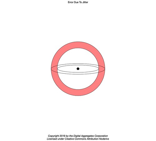
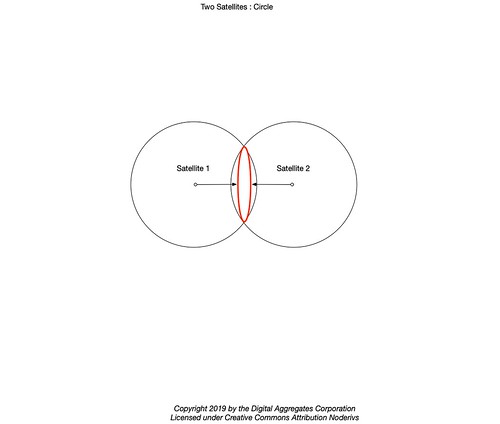
As we will see, measuring the precision of Tumbleweed is fairly straightforward. Trying to measure its accuracy dropped me down a rabbit hole from which I am still trying to extricate myself. It launched me into a self-study program into the science of geodesy:

Geodesy is the science of accurately measuring and understanding three fundamental properties of the Earth: its geometric shape, its orientation in space, and its gravity field— as well as the changes of these properties with time. [NOAA]

It also unexpectedly required that I learn a little bit about surveying:

Surveying or land surveying is the technique, profession, art and science of determining the terrestrial or three-dimensional positions of points and the distances and angles between them. A land surveying professional is called a land surveyor. These points are usually on the surface of the Earth, and they are often used to establish maps and boundaries for ownership, locations, such as building corners or the surface location of subsurface features, or other purposes required by government or civil law, such as property sales. [Wikipedia]

To fully appreciate how deep this rabbit hole is, a little context is in order.

Background

Positions on the Earth are traditionally measured in terms of latitude and longitude.

Latitude is the number of degrees north or south a location is from the Equator. The Equator is the circumferential waist of the Earth as defined by its axis of rotation. While there might be come variation about where exactly the Equator is - its position drifts about nine meters or thirty feet per year as the Earth wobbles - it is a natural reference point from which to measure latitude. The Equator is zero degrees (0°). and is a great circle: a circle whose plane passes through the center of the Earth (a position that is, however, not nearly so well defined as you might think). Locations north of the Equator are between 0° (the Equator) and 90° north (the North Pole), and locations south of the Equator are between 0° and 90° south (the South Pole). (Sometimes southern latitudes are represented as negative values.)

Longitude has no such natural reference. The arbitrary establishment of a Prime Meridian, the meridian or circumferential line (also a great circle) from the North Pole to the South Pole which defines zero degrees longitude, was, for a long time a matter of heated debate during the Age of Sail. And also, it must be said, of national pride amongst the seafaring superpowers that depended on accurate compasses, maps, and clocks in order to navigate with sufficient skill to loot the New World and enslave its inhabitants.



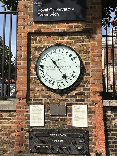
In 1884, the Prime Meridian was established by international treaty as running through the Royal Observatory in Greenwich England. The Royal Observatory was one such place where astronomical observations were made with sufficient accuracy to set clocks that could be used to navigate at sea, using them to measure longitude comparing the time on the clock on board a ship with local noon, when the Sun was at its highest point in the sky, or with other astronomical objects like the North Star.



This Prime Meridian was the standard for many decades, despite the disgruntled French who thought the Prime Meridian should run through Paris. Locations east of the Prime Meridian are said to be between 0° and 180° east, and locations west are between 0° and 180° west. (Sometimes western longitudes are represented as negative values, although in some contexts I have seen eastern longitudes represented negatively.)



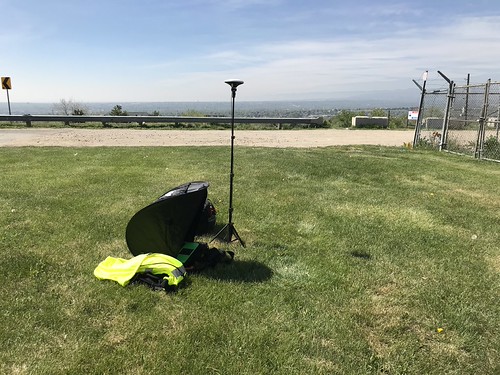
In 1973, the International Earth Rotation and Reference Systems Service (IERS), the same organization that inserts and potentially removes (although that has never happened) leap seconds into the accepted definition of Universal Coordinated Time (UTC) to keep clocks in sync with changes in the rotation of the Earth, established a new Prime Meridian. It based this new Prime Meridian on the latest scientific data at the time, much of it based in satellite observations, regarding the shape of the Earth and its center of gravity. This new Prime Meridian, which is also the GPS Meridian, is on a lawn about one hundred meters east of what is now referred to as the Greenwich Meridian, where I am standing in the photograph above, with the GPS Test Plus app on my iPhone. (Photo credit: Mrs. Overclock.)



The Greenwich Meridian, where I took the screenshot above, is about six seconds longitude west of the GPS Meridian.

Latitude and longitude are not the only coordinate systems in broad use today. The U.S. military uses the Military Grid Reference System (MGRS). This system lays down a grid of equal sized squares, the standardized size of which depends on the resolution of the map in question. MGRS lacks the sometimes problematic effect that longitude lines get closer together as you approach either pole, so that the distance between degrees of longitude ranges from just over 111 kilometers at the Equator to zero at either pole. (Degree of latitude are always sixty nautical miles apart by definition.) Many GPS receivers can be switched to display using MGRS.

While latitude and longitude are commonly used in civilian applications, including land surveying and sea navigation, there are different systems used for measuring latitude and longitude, and these systems do not yield the same results. This is due to the fact that they use different models, or datums, of the shape of the Earth. Things would be far simpler if the Earth were perfect sphere. And indeed, for short-ish distances, such an assumption served ancient mariners well. But the Earth is an oblate spheroid or ellipsoid, bulging with middle-age spread at its Equator, and flattened at either pole with the geodesic equivalent of male pattern baldness.

In 1901, the geodetic center of the United States was defined by the U.S. National Geodetic Survey (NGS), an agency of the U.S. government established in 1807, to be on Meade's Ranch, Kansas, a location that is today on private property. Since then, all land surveying in the continental United States has been done relative to this marker. Every single surveyed location is traceable through a chain of surveyor measurements and established benchmarks that eventually lead to the marker at Meade's Ranch.

In time, the NGS defined the North American Datum of 1927 (NAD27). You still see references to this abstract model of the shape of the earth and its center of gravity in old surveying documents today.

In 1983, a new, more accurate datum, NAD83, was adopted by the NGS. It was based on far more accurate measurements, mostly done from satellite observations, and it became the standard for all surveying in the United States today. (In between NAD27 and NAD83 there were other datums, just as one day, perhaps relatively soon, NAD83 will be replaced with an even more accurate datum.)

NAD83 is based relative to the North American tectonic plate. Because the North American tectonic plate moves at a rate of over two centimeters per year (and the Pacific plate, on which part of California sits, as much as seven to eleven centimeters per year), measurements made using NAD83 do not change (much) as the tectonic plate takes its leisurely stroll over a thick layer of lubricating rock.



"Much" because the NGS survey markers - typically inscribed cast metal disks embedded in concrete pillars or in sidewalks - are often embedded in ground which moves relative to local landmarks just due to smaller, local shifts in the ground. Or, as I like to say, "Shift happens".



(Local municipalities will also establish their own survey markers, sometimes fiberglass embedded in concrete.)

The use of relatively local coordinate systems on which to base latitude and longitude is quite common, and especially important in locales in which there is a lot of continental drift due to tectonic movement. New Zealand resides on two different tectonic plates, the Australian plate (the North Island and the western part of the South Island) and the Pacific plate (the rest of the South Island). The Pacific plate rotates counter-clockwise compared to the relatively stable Australian plate, making surveying in New Zealand especially challenging.

In 1984, the U.S. National Geospatial-intelligence Agency (NGA) established the World Geodetic System (WGS84). This is the datum on which GPS is based. The NGA is responsible for, amongst other things, providing accurate maps to the U.S. Department of Defense. WGS84 creates yet another coordinate system, but unlike NAD83, this one one is not relative to a tectonic plate, but is instead a global coordinate system. Because WGS84 deliberately does not take plate tectonics into account, GPS coordinates of a particular location may change (slowly) over time as the continental plate drifts. But because GPS coordinates can be made so swiftly - in minutes or seconds instead of hours or days required for expensive manual surveying - this isn't generally an issue.

However, this means that the GPS coordinates - made using WGS84 - of an NGS marker - whose position was originally determined using NAD83 - cannot be directly compared. Worse yet, any conversion between WGS84 and NAD83 has to take the date the measurements were made into account in order to adjust for continental drift.

Now that we've covered all the stuff I had to learn and worry about regarding exactly what the results from measurements I did with Tumbleweed even mean, we're ready to talk about what metrics of quality I used and what tools I used to measure and analyze them.

Quality Metrics

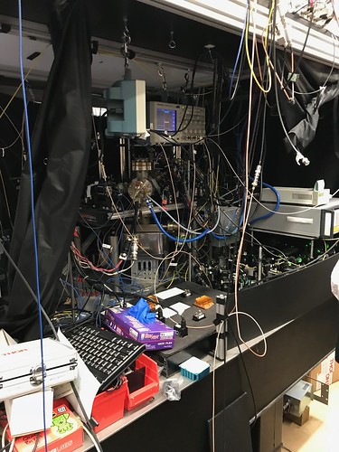
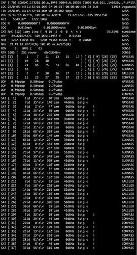
The gpstool command line utility is the Swiss Army knife of Hazer. It parses the output of the ZED-F9P module using the functions in libhazer: National Marine Equipment Association (NMEA) 0183 sentences, the most typical output of GNSS receivers, are parsed by the Hazer functions; proprietary u-blox binary messages in UBX are parsed by the Yodel functions; packets conforming to the Radio Technical Commission for Maritime Services (RTCM) Special Committee (SC) 104 standard are parsed by the Tumbleweed functions.

When used with the ZED-F9P (and many other u-blox GNSS receivers), gpstool configures the module to emit the proprietary High Precision Geodetic Position Solution (UBX-NAV-HPPOSLLH) message, a UBX message with a higher precision latitude, longitude, and altitude than is typically available via NMEA. The message also includes a Horizontal Accuracy Estimate and a Vertical Accuracy Estimate in units of one-tenth of a millimeter. How these estimates are computed isn't documented (that I've found). But it is plausible that the ZED-F9P could base these metrics on how closely it was able to bring the range spheres using the iterative least squares algorithms before the range spheres began to move away.

HPP   39.821674271 -105.095174932 ±     0.0141m
HPA   1722.1183m MSL   1700.5934m WGS84 ±     0.0100m

The High Precision Position (in decimal degrees) and the High Precision Altitude (in meters), along with the accuracy estimates (in meters), are displayed in real-time by gpstool as the HPP and HPA output lines. The HPA line includes both the altitude above Mean Sea Level (MSL) and above the WGS84 ellipsoid (WGS84). The HPP line is formatted such that the coordinates can be cut and pasted directly into Google Maps. The example above is from an actual field test of a Tumbleweed Rover receiving differential corrections from a Tumbleweed Base.

The Horizontal and Vertical Accuracy Estimates provide a self-reported metric of quality for the ZED-F9P, although since the module doesn't know what the actual coordinates are, I'm not sure you can actually call these metrics a measure of "accuracy". But given that uncorrected GPS under the best circumstances is accurate to about five meters or about fifteen feet, and under poor circumstances a lot worse, small numbers for these metrics are a good thing. Note in the example above that the horizontal accuracy estimate is 1.41 centimeters (a little over half an inch), and the vertical accuracy estimate is 1.00 centimeters (less than half an inch).



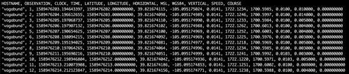
gpstool has the option (-T) of appending each instance of the high precision solution, along with the GPS Time, to a Comma Separated Value (CSV) file. The ZED-F9P is configured by gpstool to emit a high precision solution once a second (one hertz). The CSV file simplifies analysis with Excel or other tools, especially when looking at how the position solution changes over time.

The geodesic command line utility in Hazer computes the shortest distance between two sets of latitude and longitude coordinates as measured on the surface of the WGS84 ellipsoid. It is implemented using code borrowed from the GeographicLib library developed by Charles F. F. Karney and licensed under the MIT/X11 License. geodesic is useful for comparing coordinates generated with Tumbleweed with those from other sources like professional differential GNSS hardware and from NGS benchmarks, and can be used to assess both the precision and accuracy of the device.

The haversine command line utility in Hazer is similar to geodesic except that it uses the simpler Great Circle Route algorithm, from spherical trigonometry, that assumes that the Earth is a perfect sphere. For small distances it produces comparable results. For large distances, the output of the two utilities typically differ significantly. (I haven't used haversine since I wrote geodesic.)

The csvlimits command line utility in Hazer reads a CSV file from standard input and displays the minimum longitude value, the minimum latitude value (not necessarily from the same sample), the maximum longitude value, and the maximum latitude value (ditto). These values form the opposite corners of a square which bounds all of the latitude and longitude coordinates in the CSV file. It can also be thought of as a diameter defining a (slightly larger) circle. All of the positioning solutions will fit within the square/circle. Using the geodesic utility on these synthesized minimum and maximum coordinates gives a measurement of the precision of the module in different circumstances when it is stationary.

The csv2kml command line utility in Hazer reads a CSV file from standard input and converts it into a Keyhole Markup Language (KML) file which it emits to standard output. KML is an XML-based language that is understood by Google Earth. This allows you to take the CSV output from gpstool and visualize it graphically on top of actual satellite imagery of the Earth's surface. This can be used to assess both the precision and the accuracy (as it compares with Google Earth) of the device.

The NGS NGSDataExplorer is a web-based tool that gives you access to the NGS online database of documented survey markers. The tool provides a graphical map location of the marker and access to the official data sheets describing the marker, its location, and how it was surveyed. This can be used, with some conversion, to compare the NGS coordinates with that of the device.

The National Oceanographic and Atmospheric Administration (NOAA) Horizontal Time Dependent Positioning (HTDP) web-based tool converts between geodesic coordinate systems like NGS83 and WGS84, taking the time the measurements were made into account. This allows you to assess the accuracy to the device by comparing its output with the coordinates of, for example, an NGS survey marker.

The mapstool command line utility in Hazer coverts coordinates in a variety of formats, including those used in the NGS data sheets, into a decimal degrees form that can be used with geodesic, HTDP, Google Maps, and Google Earth.

The Tumbleweed Base is somewhat arbitrarily (by me) configured to survey-in to an accuracy of 2.5 centimeters or just less than an inch; it looks days of uninterrupted geolocation for the long term weighted average of the positioning solution to converge to that accuracy. The duration (or even success) of the Base survey depends greatly on antenna placement. A survey with marginal antenna placement, if successful at all, can take several days. (I'll talk more about that in a later article.) The Base surveyed into the following coordinates.

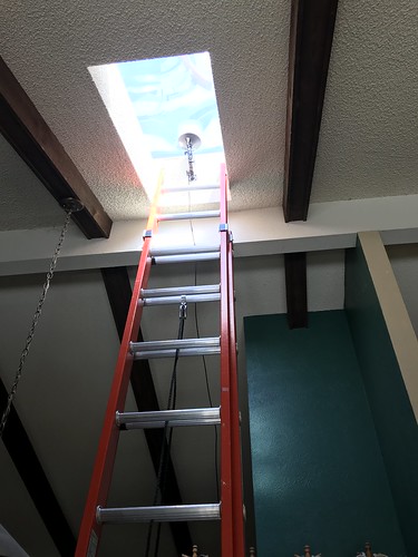
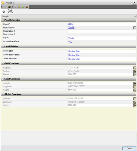
High Precision Position: 39.794275645, -105.153414843

Horizontal Accuracy Estimate: 0.0204m

High Precision Altitude: 1708.4968m MSL 1686.9969m WGS84

Vertical Accuracy Estimate: 0.0144m



These are the coordinates of the skylight above my kitchen, near the peak of the roof, although Google Maps places it just to the upper left of the skylight. Whether this is a measurement error in the survey-in process or some slop in Google Maps is an open question.

Precision and Absolute Accuracy

I measured precision and absolute accuracy using NGS marker KK1446 "Dover". "KK1446" is the marker's Persistent Identifier (PID) and "Dover" its designation (it's off a street named Dover Way). KK1446 is set in a small field next to a fenced off municipal water tank at the edge of a suburban housing development in Arvada Colorado. It was established in 1977 and resurveyed in 1993 at the following NAD83 coordinates (shown in the NGS hour minutes seconds data sheet format).

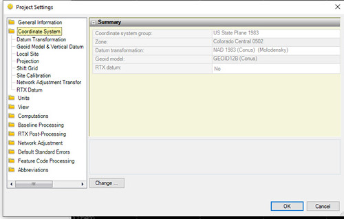
39 49 17.98157(N) 105 05 42.59638(W)

HTDP converts those NAD83 coordinates into following WGS84 coordinates (also in NGS data sheet format).

39 49 17.99968(N) 105 05 42.64410(W)

mapstool converts those coordinates from NGS data sheet format into decimal degrees.

39.821666578, -105.095178917

The stationary Rover antenna was centered directly over the KK1446 and twenty minutes of data was collected, yielding over a thousand data points in the CSV file. Precision was determined using csvlimits and geodesic to compute the diameter of the enclosing circle (or square). Absolute accuracy was determined using geodesic to compute the distance between the coordinates of the marker (converted into WGS84) and the high precision position determined by the ZED-F9P.

Two tests were run: one using corrections from the Base, and one with no corrections. The CSV files from each test were converted using csv2kml and imported into to Google Earth. The corrected test run is precise enough that you'll need to click on the images to see a larger version in order to see the red plot made by Google Earth; blowing up the images any more blurs the detail.

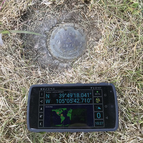
Date: 2020-05-14

Location: NGS KK1446

Configuration: Corrected Rover

High Precision Position: 39.821674271, -105.095174932

Horizontal Accuracy Estimate: 0.0141m

High Precision Altitude: 1722.1183m MSL 1700.5934m WGS84

Vertical Accuracy Estimate: 0.0100m

Precision: 0.0423m

Accuracy: 0.9198m

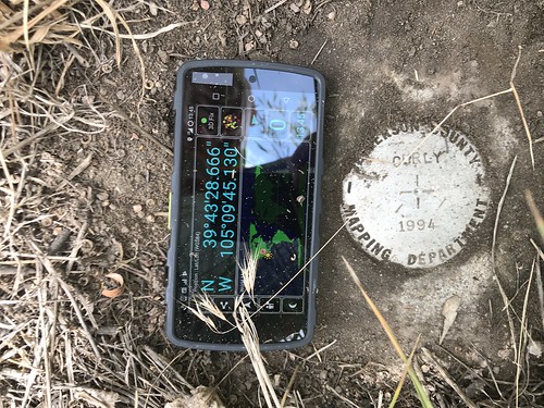
Date: 2020-05-18

Location: NGS KK1446

Configuration: Uncorrected Rover

High Precision Position: 39.821671099, -105.095169044

Horizontal Accuracy Estimate: 0.4327m

High Precision Altitude: 1724.6724m MSL   1703.1475m WGS84

Vertical Accuracy Estimate: 0.6372m

Precision: 0.6925m

Accuracy: 0.9831m

The precision - the diameter of the circle in which all of the position solutions lie - of the corrected Rover test is a little over four centimeters. This is not as good as I had hoped (my original goal was to get within 2.5 centimeters or about an inch), but far better than the uncorrected precision which was almost seven-tenths of a meter or more than two and a quarter feet.

The accuracy - how far the computed WGS84 coordinates differ from the surveyed NAD83 coordinates converted to WGS84 - of the corrected Rover is not that great: nine-tenths of a meter, and not that much better than the uncorrected Rover.

Since I don't know exactly how the ZED-F9P computes its own accuracy estimates, I'm not sure how to compare them with my own quality metrics.

I would be tempted to blame the multi-step conversion process I used to get WGS84 coordinates of KK1446 that I could directly compare with my own results, had not a chance meeting occurred.

Comparative Accuracy



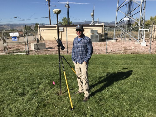
During one of my field tests in October 2019 I discovered I wasn't the only person that liked using NGS KK1446 for testing their GNSS equipment: I had to share the spot with a professional surveyor who showed up to check his own equipment as part of a job. He very graciously shared the results from his high-zoot survey-quality Trimble GNSS with me. I confess to a certain amount of equipment envy.



One of the advantages of professional equipment is his Trimble displayed its GNSS measurements using the NAD83 datum, standard in the surveying field, instead of WGS84, the standard for GPS.



Taking the Trimble's NAD83 coordinates, using the HTDP web tool to convert them to WGS84 coordinates, then using geodesic to compute the distance between those coordinates and the KK1446 coordinates converted to WGS84 (because geodesic assumes WGS84) yields a difference of 0.0307 meters or about three centimeters. That's very good, and far better than what I've been able to achieve.

Relative Accuracy



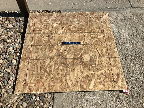
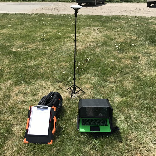
I measured relative accuracy by building a test fixture. I used a sheet of plywood on which I marked off, as carefully as I could with a square and a meter tape, one square meter. I got the board approximately level using a torpedo level and some makeshift leveling blocks.



I set my Rover in its sunshade and on its stand on the board (which wasn't really necessary for the results, but allowed me to reach all four corners of the meter square without using more coax cable). I collected five minutes of data at each corner, keeping the antenna as motionless and level (using a circular level built into the pole) as possible. I repeated the cycle of all four corners twice.

The geodesic measurement between successive corners ranged from 0.9810 meters to 1.010 meters with a mean of 0.9939 and a standard deviation of 0.0101 (computed using Excel). That's pretty good; much of the variation may be a result of my own inability to lay out a perfect square meter on a sheet of plywood and to hold the survey pole with the antenna steady while my neighbors watch me with their usual curiosity. My original goal was an accuracy of 2.5 centimeters or about an inch, and this falls well within that.

Negative Results Are Still Results

The title of this article came from a remark my thesis advisor Bob Dixon made thirty-seven years ago, when I was working on my master's thesis in computer science at Wright State University in Dayton Ohio.

My original goal for this project was to see if consumer grade differential GNSS technology was precise enough for applications like agriculture: self-navigating tractors, etc. The results indicate that the ZED-F9P is indeed capable of precise, self-consistent, repeatable geolocation, and that the use of differential corrections from a base station also equipped with a ZED-F9P makes a significant measurable difference.

I was disappointed in its accuracy results when trying to duplicate the coordinates of surveyed markers like KK1446. There are a lot of reasons why this lack of accuracy may have been the case, although the success of the Trimble in this regard makes me think better accuracy should be achievable (and that you get what you pay for). It's possible that I need a better antenna, or that there's a mistake in my own calculations. (While some of the tools I wrote for Tumbleweed use double precision floating point, gpstool and the functions it uses in libhazer that parse the output of GNSS devices use only integer arithmetic, even though the displayed values may appear to be decimal. I have also tried to keep track of the significant digits in various internal calculations.)

I keep alluding to the important of antenna selection and placement in achieving good results with GNSS, whether or not differential corrections are being used. This will be the topic of an upcoming article.

Acknowledgements

Thanks to Charles Karney, who wrote GeographicLib and open sourced it, and of which I used only a tiny part in my geodesic computations.

Thanks to Brad Gabbard of Flatirons, Inc., a surveying, engineering, and geomatics firm based in Boulder Colorado, who graciously put up with the old guy and his a tub of improvised equipment, and who so generously shared his results with me.

Frames of Reference IV

Einstein's Theory of Special Relativity tells us that the faster you go, the slower time passes. It stops passing at all at the speed of light.

Einstein's Theory of General Relativity tells us that the closer you are to a mass, or the more massive that object is - meaning, the deeper you are in a gravity well, because gravity is a property of mass - the slower time passes. It stops passing altogether inside a black hole.

It would be easy to think that these ideas are just hypothetical. But they're not. These effects have been almost trivially observed, just by taking extremely accurate clocks in airplanes or to the tops of mountains and back, and then comparing them to equally accurate clocks with which they were synchronized beforehand. The differences in the clocks matched the predictions made by Einstein's equations.



The extraordinarily precise ytterbium (Yb) lattice optical atomic clock at the National Institute of Science and Technology (NIST) laboratory in Boulder Colorado, a portion of which is shown above, measures the passage of time by taking measurements finer than the width of a hydrogen atom. It is so precise, that its output is measurably affected by a change in its vertical position from the Earth's mass of just a few centimeters.

The scientists responsible for the clock had the laboratory floor officially surveyed to determine its altitude with as much accuracy as humanly possible. That's the National Geodetic Survey (NGS) benchmark embedded in the lab floor.

The Global Positioning System (GPS) falls prey to both of these effects: orbits are a form of centripetal acceleration - satellites in orbit are continuously falling but just miss the Earth; and satellites in orbit are further away from the Earth's mass than objects on the ground. GPS depends on atomic clocks in each satellite to work. Special Relativity causes the clocks to run slow by about 7 microseconds a day relative to a clock on the ground. General Relativity causes those same clocks to run fast by about 45 microseconds a day relative to a clock on the ground. The net effect is that the GPS clocks run fast by about 38 microseconds a day.

The GPS system had to be designed to take this into account. Light - and, hence, the signals from the GPS satellites - travels almost 300 meters in a microsecond, or almost 1000 feet. Being off by 38 microseconds means positioning calculations made by your GPS receiver would be off by 38,000 feet, or more than seven miles, if the effects predicted by Special Relativity and General Relativity weren't taken into account.

Every object in the Universe - the device you're reading this on, a boulder on the planet Mars, all of the atoms in your body - is exposed to a slightly different gravity field, just by virtue of being in a slightly different place relative to all of the other objects in the Universe.

That means every object in the Universe experiences time a little differently than every other object. When you're standing, time passes more slowly for your feet than for your head just because your feet are closer to the mass of the Earth.

The cells on top of your foot experience time differently than the cells on the bottom of your foot.

The molecules at the top of a cell in your foot experience time different than the molecules at the bottom of that same cell.

The atoms in that molecule that are further from the Earth experience time differently than the atoms in that same molecule that are closer to the Earth.



There is no one time that everyone shares. Every single object has its own time, running faster for some, slower for others.

Sources

Richard W. Pogge, "GPS and Relativity", Ohio State University, 2017-03

Carlos Rovelli, The Order of Time, Riverhead Books, New York, 2018

Practical Differential Geolocation

Today, I have seven Global Navigation Satellite System (GNSS) antennas in the window of my home office at the rear of our house. I have an eighth one in the window of our living room in the front of the house. A ninth one in the skylight near the peak of the roof above our kitchen. And a tenth one sitting on my lab bench. All of these are hooked up to active GNSS receivers.

This isn't as crazy as it sounds. Five of those are used, not for geolocation, but for precision timing, disciplining the clocks in Network Time Protocol (NTP) servers. Two are used to continuously monitor the various GNSS constellations. Two are for functional and regression testing my own software. And one is connected to the base station for my Differential GNSS project. Differential GNSS (or, formerly, Differential GPS) is another approach for squeezing more accuracy and precision out of the GNSS constellations for Positioning, Navigation, and Timing (PNT) applications.

Differential GNSS

In Pseudorange Multilateration and Dilution of Precision I talked about just some of the ways errors are introduced into the GNSS position fix solution, and some of the mechanisms through which these errors can be addressed. In Improvisational Engineering I touched on another technique that uses corrections transmitted from a fixed base station to a mobile rover.

Differential GPS - or, again more generally, Differential GNSS - takes advantage of the fact that the sources of error (typically jitter) in the received satellite signals are uncorrelated with one another. Which is to say: random, or at least not systemic. So if a GNSS receiver is stationary, it can take advantage of its fixed location to compare each successive solution with either its own predetermined location, or with its own long term weighted average positioning solution. In the latter technique, called Real Time Kinematics (RTK), the receiver's position solution can become more and more accurate over time. Depending on a number of factors like antenna placement and how many satellites it can see overhead at a time, a stationary receiver, or the Base in DGNSS parlance, can achieve an accuracy down to centimeters or better.

This sounds great, but it doesn't help the mobile receiver, or Rover. Except if the Rover is close enough to the Base - in the same neighborhood - the two receivers will see the same satellites overhead, and therefore suffer similar degradation in the signals. The Base can transmit its corrections to one or more Rovers, and each mobile Rover can then potentially achieve a similar level of accuracy. 

DGNSS products have been around for decades, costing on the order of thousands of dollars. Late in 2018, u-blox, the well known Swiss-based manufacturer of excellent (in my professional experience) PNT solutions, introduced their ninth-generation of GNSS receiver chips, the ZED-F9. This family of high-precision GNSS chips support DGNSS RTK directly, in the form of messaging conforming to the Radio Technical Commission for Maritime Services (RTCM) Special Committee (SC) 104 standard. This brings a DGNSS capability down to a price range of hundreds of dollars, potentially affordable to hobbyists, enthusiasts, experimenters, and consumers of applications like non-military drones and remotely piloted or autonomous vehicles.

...

I have been using u-blox PNT solutions for years professionally. And the National Center for Atmospheric Research (NCAR) in Boulder Colorado had an R&D group decades ago when I worked there that was using DGNSS that was good enough that they could measure the swinging of instrument packages tethered to high altitude weather balloons. So when I first read about the ZED-F9 on the Time Nuts mailing list, my ears perked up.

The corrections generated by the Base are made on the assumption that the Base is stationary, so that any differences between its latest computed solution and its known location must be due to timing variations in the received signals. Because the Rover is moving, it cannot make any such assumptions. But as long as the GNSS receivers in both the Base and the Rover are seeing the same signals, the Rover can take advantage of the Base's corrections.

Differential techniques like this have been in use for a long time. Early versions required that the position of the Base be established through meticulous manual surveying.

Then consumer GPS and GNSS receivers began to support a survey-in mode in which the Base established its own position over time (hours or even days) to a required level of precision. But this still required a substantial amount of software development to implement the RTCM stack or equivalent messaging.

Today, there are a variety of established augmentation systems, ranging from fixed reference stations to even geosynchronous satellites, that provide differential corrections. Most of them are specific to the GPS constellation. Some of these are already automatically used by GPS receivers. Some of them are commercial services that you pay to subscribe to. Some of them aren't that useful.

The big breakthrough for folks like me came when affordable GNSS modules like the ZED-F9P came on the market, supporting RTCM SC 104 messaging natively, either providing corrections via RTCM after completing a survey-in, or accepting those corrections, even from some other RTCM source than another ZED-F9P module, and applying them in real-time to its own positioning solution. The ZED-F9P was also highly configurable in both hardware and firmware, able to be adapted to use a variety of communication ports to provide and accept RTCM messaging.

To be clear: virtually everything I have done on this project is merely glue code. It is the firmware in the ZED-F9P that does all the heavy lifting.

Background

(You can click on any image to see a larger version.)



I have been experimenting with affordable consumer GPS receivers that provide a computer interface (typically USB) for a few years. This resulted in Hazer, my open source Linux/GNU/C-based software stack to parse and interpret the National Marine Electronics Association (NMEA) 0183 standard messages generated by most GPS receivers. Hazer provides a libhazer containing functions to handle NMEA, and a gpstool utility that can be used to functionally test it. Hazer can be found in the repository com-diag-hazer on GitHub.



I had encountered u-blox GPS receiver modules professionally on various embedded product development projects a decade before I began working on Hazer. When I started trying receivers with later generations of u-blox modules with Hazer, I expanded my support for those devices by adding Yodel, a parallel software stack in the Hazer repository, that handles messages in the proprietary UBX protocol, used by u-blox to provide more complex capabilities. gpstool evolved to not only handle the real-time configuration of these devices using UBX, but to incorporate features that supported experiments like integration with Google Earth for a real-time vehicle tracking.



When I started playing with the ZED-F9P module a year ago, I added Tumbleweed, yet another parallel software stack in the Hazer repository, that provides basic support for RTCM SC 104 messaging. I also added the rtktool utility that handles the routing of RTCM corrections from a Base to any number of Rovers across the internet.

Theory of Operation

This is the architecture into which Tumbleweed has evolved.



The Base is a Linux/GNU host that runs gpstool, a process which communicates with a USB-attached ZED-F9P module. Following a successful period of surveying in, the ZED-F9P establishes its fixed location to a configured level of accuracy. It then begins to transmit RTCM corrections to the host via USB. gpstool forwards the RTCM corrections via User Datagram Protocol (UDP) to the RTK Router.

The Router runs rtktool, a process which listens on a well known UDP port for incoming RTCM messages. These messages can either be corrections from the Base, or empty messages that serve as keep alive messages from one or more Rovers.

When the Router receives its first RTCM correction from a Base, it registers the IP address and UDP port number for that Base as the sole source for RTCM corrections. Any subsequent corrections from other Bases are ignored until the original Base quits transmitting corrections and its registration times out. Then the next Base whose corrections are received has its IP address and UDP port number registered as the source of RTCM corrections.

The Rover periodically sends an RTCM message with no payload to the Router via UDP as a keep alive. They are sent frequently enough to prevent the Router from aging out the Rover's IP address and UDP port number from its cache. The Rover receives RTCM corrections via UDP, addressed by the Router to the IP address and port number in its cache. gpstool forwards the RTCM corrections to the ZED-F9P via USB.

When the Router receives an empty RTCM message via UDP from a Rover whose IP address and UDP port number it does not already have in its cache, it adds that information to the cache. When the Router receives an RTCM correction from the one and only Base, it forwards that correction to any and all Rovers in its cache via UDP. If the Router does not receive a keep alive from a Rover within a time out period, the information for that Rover is removed from the cache.

In my implementation at the Palatial Overclock Estate, the Base sits on my home WiFi network, communicating wirelessly with the Router. The Router has a direct wired connection to my home WiFi access point/router, and forwards RTCM corrections to Rovers via our home internet service provider. Rovers in the field use a USB-attached cellular modem, and send keep alives and receive corrections via my LTE mobile provider.

The architecture is agnostic as to the communication mechanism, as long as it supports UDP/IP.

Useful variations in the architecture are possible.

This simpler scheme combines the Base and the Router by simply running gpstool and rtktool on the same Linux/GNU host. I have used this approach, but it didn't turn out to be convenient for my physical setup, which will be shown below.

Issues

There are a few details of which anyone trying to duplicate this setup should be aware.

The use of UDP instead of the guaranteed reliable Transmission Control Protocol (TCP) is important. As I discussed in the article Better Never Than Late, real-time applications like this become dysfunctional when messages arrive too late. RTCM corrections that arrive too late are useless. Not only do they have to be discarded by the receiver if they arrive after their "expiration date", the presence of useless messages in the pipeline delays the more applicable messages that are waiting behind the clog, often making them too late to be useful.

I routinely observe dropped messages, and occasionally out-of-order messages, particularly on the relatively complex Router to Rover link. When I initially did testing using TCP with Hazer prior to Tumbleweed, clogging of the data path and delayed messages were also routinely observed.

The Base prepends its outgoing RTCM messages with an unsigned thirty-two bit sequence number, as does the Rover. This allows the Router and the Rover to discard out of order messages, and to detect when messages have been dropped.

Never the less, the use of UDP is problematic. There is no authentication between the Base and Router, or between the Router and Rover. This means Denial of Service (DoS) attacks, spoofing, or other mischief are trivially possible. There is no encryption either, which could reveal sensitive location information.

However, usable encrypted UDP is an unsolved problem in my opinion. The obvious solution, Datagram Layer Transport Security (DLTS), works in part by implementing packet ordering and retransmission, effectively providing TCP-like services on top of UDP. This defeats the purpose of using UDP in the first place, bringing with it all the real-time problems of TCP.

Authentication and encryption are issues I am still pondering. I am frankly hoping someone else eventually solves this problem for the general UDP case.

The Router is necessary because none of the Linux/GNU hosts in Tumbleweed - Base, Router, or Rover - have static IP addresses. As is typical, my internet service provider dynamically assigns an IP address via Dynamic Host Configuration Protocol (DHCP) to my home WiFi access point/router. IP packets to and from hosts on my home network, like the Base and the Router, are routed though a firewall that does Network Address Translation (NAT).

Similarly, the Rover is dynamically assigned an IP address via DHCP by my LTE mobile provider. To further complicate matters, testing in the field has shown that the Rover's IP address (or sometimes just its UDP port number), once established, can be dropped and a new, different, one assigned, by my mobile provider, perhaps as a result of cell site handover; this happens even when the Rover is stationary.

I subscribe to a Dynamic DNS (DDNS) service. My home access point/router supports DDSN directly. When it boots and is assigned an IP address by my ISP via DHCP, the device automatically notifies the DDNS service of this fact, and the DDNS service then updates the global DNS database so that a fixed internet domain name points to this address. This, plus a firewall rule configured into my access point/router, allows me use a fixed domain name to point to the RTK Router when I start up a Rover. (The Base simply uses a local static IP address for the Router that is only valid behind the firewall.)

If the Rover's IP address and/or UDP port changes while it is being used in the field and receiving corrections, the next time it sends a keep alive to the Router, its IP address and UDP port number will be cached by rtktool as a new Rover, and it will receive the next RTCM correction using this new information. The entry with the old IP address and UDP port number will eventually become stale and be removed from the cache by rtktool. In the meantime, some RTCM corrections may be sent to the old address, but will presumably be dropped by the network.

(Another problem with the lack of authentication and encryption is that those orphaned RTCM corrections can actually be delivered to some unrelated host that has an application that just happens to be listening to the same UDP port. Other distributed systems I've helped develop do not immediately reuse dynamically assigned IP addresses for exactly this reason.)

Practical Differential Geolocation

This is the Tumbleweed setup I'm using today. It took me a long time to arrive at this specific setup, as I related in Improvisational Engineering. Some of this will convince you that Mrs. Overclock is a remarkably understanding woman.



This is the fixed Base station running gpstool. It is hidden in a drawer of a narrow dresser tucked inconspicuously into the corner of our living room. The host is a Raspberry Pi 3B+ Single Board Computer (SBC) running Raspbian, a Linux/GNU distro derived from Debian. The SBC is inside a plastic enclosure with a fan. A SparkFun GPS-RTK2 board with a u-blox ZED-F9P module is connected to the host via USB. The Base is plugged into an Uninterruptible Power Supply (UPS) hidden in another drawer below it.



This is the survey-grade multi band GNSS active antenna. It is mounted on a wall mount intended for a security camera in a skylight above our kitchen. The skylight is very near the peak of that section the roof, so the antenna has a good view of the sky. A small coaxial cable snakes down from the antenna and crosses a low wall from the kitchen into the living room to enter the dresser adjacent to the wall from the rear.



The Base runs headless - that is, without a monitor, keyboard, or mouse - but the output from gpstool can be viewed on demand when using ssh to log into the host across our home network. Here, gpstool shows that the ZED-F9P self-reported a horizontal position accuracy of 0.0204 meters (a little less than an inch) and a vertical position accuracy of 0.0144 meters (a little more than half an inch). It used twenty-five different satellites from all four GNSS constellations (GPS a.k.a. NAVSTAR, GLONASS, Galileo, and Beidou a.k.a. COMPASS) for its position solution. On at least one occasion since gpstool was last started, the ZED-F9P was able to use a maximum of thirty-two satellites for a solution.



This is the Router running rtktool. Is is a similar Raspberry Pi 3B+ SBC running Raspbian. It has no special hardware. You can see the plastic enclosure with the fan running, but not much else. It is tucked into a shelf of our A/V cabinet in our family room (right where the cable from our ISP enters the house) where it is directly connected via a CAT5 cable (visible as the yellow RJ45 connector) to our home WiFi access point/IP router in the same cabinet. Like much of the stuff in our A/V cabinet, the Router is powered via a UPS.



This is a Rover running gpstool. It is a CEED pi-top [3] laptop shell. The pi-top [3] looks like a laptop, with a display, keyboard, and trackpad, but it has no internal processor, memory, or storage. Attached to the Rover is another survey-grade multi band GNSS antenna. The antenna is mounted on a selfie-stick intended for small cameras and mobile phones.



Sliding the keyboard and trackpad bezel down reveals the guts of the pi-top [3]. It has a glue board, heat sink, and system connector that accommodates a Raspberry Pi 3B+ SBC. (The SBC is hidden under the silver heat sink/system connector.) On the right, connected via a USB port on the glue board, is another SparkFun GPS-RTK2 board with the ZED-F9P module. The board is attached magnetically to an accessory rail. All of this fits, hidden, underneath the keyboard and trackpad bezel when it is closed.



On the rear of the pi-top [3] to the left is an SMC connector to which the GNSS antenna is attached. (I drilled a hole for that.) On the right on an external USB port is a NovaTel USB730L global LTE modem. This device enumerates to its host as an Ethernet dongle and self-configures by acting as a DHCP server to the host; all of the mobile network functions are hidden.



This is the Rover in the field, peeking out from underneath a laptop sunshade, geolocating over U.S. National Geodetic Survey (NGS) marker KK1446 near my neighborhood.



During this same field test, gpstool indicates that the ZED-F9P self-reported a horizontal accuracy of 0.0141 meters (a little over half an inch) and a vertical accuracy of 0.0100 meters (less than a half an inch). It was using twenty-eight different satellites from four different GNSS constellations for its position solution, and had used twenty-nine satellites at some time since gpstool had started.



Although the Raspberry Pi is my go-to SBC for projects like this, the software isn't married to it. Here is a second Rover that I stood up. It is an ancient HP Mini 110 netbook running Linux Mint, another Linux/GNU distro based on Debian. This tiny laptop has a 32-bit Intel Atom N270 i686-class processor. Plugged into a USB port on the left, you can see another USB730L LTE modem. Plugged into a USB port on the right, inside a 3D printed enclosure, is an Ardusimple SimpleRTK2B board which also has a ZED-F9P module. Attached to the GNSS receiver is a helical GNSS antenna. This laptop, which a friend of mine accurately described as "dirt cheap and dead slow", is running gpstool and differentially geolocating like a boss, the u-blox module doing all of the heavy lifting.

Results

One of the challenges I had when I built my own NTP server with a cesium atomic clock was: how do I test a device that may be far more accurate/precise than any tool I have with which to test it? I feel like I more or less solved that problem for the clock, at least to my own satisfaction. What kind of real-world results can I expect from Tumbleweed? How will I know that it even works?

That is a topic for another article.

Updated (2020-09-21)

I recently re-ran the long term survey-in of my Base station. The survey-in took a little over eight days to arrive at my desired mean accuracy of 2.5 centimeters or a little less than an inch. Here is a graph of the mean accuracy over the survey-in duration in seconds.

This is pretty much what I expected: the mean accuracy converges with a long tail.

Dilution of Precision

In Pseudorange Multilateration I described the basics of how the Global Positioning System (GPS) works, but left out some of the gory details. Here are some of the gory details, again at my dilettante level of understanding.

More Is Better

When your GPS receiver calculates the range to a GPS satellite, we tend visualize that computation as the receiver resting somewhere on a sphere defined by the space vehicle at the center and the radius being the range. The receiver doesn't know where on the sphere it resides. But all points on that sphere are equidistant from the satellite.



But that visualization doesn't really capture the reality of the situation. Because there is inevitably some variation or jitter in the timing of the signal from the satellite, the situation is more accurately visualized as a sphere within a sphere. The two spheres represent the minimum and maximum value of the range given its uncertainty. Your receiver is somewhere in the volume that is the interstitial space between the two spheres.



We continue to mislead ourselves by visualizing the range to a second satellite defining a second sphere which intersect with the first in a circle.



But this is also incorrect. What actually happens is a second set of two nested spheres intersects with the first, reducing the volume in which the solution of the position fix may reside into the shape of a doughnut or a pancake depending on how much they overlap.



The addition of more computed ranges from more satellites keeps chopping away at this volume, as the solution lies in the intersection of all the volumes of the individual solution spaces.



This is definitely a case of More Is Better. As in: more than the four, and only four, satellites needed for the closed-form algebraic multilateration algorithm. So modern GPS receivers - like yours - instead use an iterative approach based on the least squares algorithm, handy when a problem is overdetermined: more equations (computed ranges) than free variables (X, Y, Z, and T).

Your GPS receiver feeds the algorithm as many ranges as it can compute from the satellites in view. The receiver is also tasked with synchronizing its internal clock to GPS Time, solving for X, Y and Z , its position in space, as it adjusts T. Until this is done, the computed ranges cannot be accurate. In fact, they will each be off by a billion feet for every second the internal clock differs from the time on the synchronized atomic clocks in the GPS constellation.

So the processor in your GPS receiver iterates by adjusting its clock in whatever direction causes this computation to converge. This is in whatever direction causes the intersected volume defined by the range spheres to grow smaller, with the goal to draw the spheres to intersect at a point. Eventually the volume is reduced, probably not not to zero, but to some value of T in which any additional change causes the volume to begin to grow again as the spheres move apart.

At this point, three really useful things have occurred.

First: your GPS receiver now knows its position within a volume. It's not perfect, but it's as good as it's going to get.

Second: your GPS receiver has a measure of the accuracy of its solution, in terms of the size of the minimized solution volume bounded by how far apart the range spheres are. This is a useful thing to know.

Third: your GPS receiver's internal clock is now, and continuously as long as position fixes keep coming, closely synchronized to GPS Time. This makes subsequent position fixes much faster. Should your receiver loose contact with the GPS constellation - for example, your automobile drives under an overpass (short time) or into a tunnel (long time) - whether the algorithm has to start from scratch when the GPS signals are reacquired depends on how long it was cut off and the quality of its internal clock (holdover). But even if it has drifted some relative to GPS Time, if it has not drifted much, subsequent position fixes will be must faster.

But this iterative, geometric, approach to achieving a position fix has its own issues.

Dilution Of Precision

Not all satellites are created equal. Considering the two satellite diagram above, we think of the overlap between the two solution spaces as being relatively small compared to the volumes in the two sets of nested spheres individually.

But that assumes that the satellites used for the position fix have wide physical separation. This requires a very broad view of the sky (as shown in the diagram) so that your GPS receiver can use satellites whose orbits have not placed them close together.

What if the your GPS receiver is in a canyon, perhaps an "urban canyon" between two ginormous buildings, so that it has a restricted view of the sky?



In this case, the overlap of the two solution spaces may be nearly 100%, because your receiver can only see satellites whose orbits happen to place them very close together, in that narrow slice of sky, at the time of the position fix. The addition of a second satellite does not do much to reduce the volume in which the position fix may reside. As we continue to add more ranges to the algorithm based on satellites in close proximity, the final position fix volume may still be quite large.

This is called Dilution Of Precision (DOP). DOP measures how sensitive the position solution (output) is relative to changes in the pseudo-ranges (input). The closer the satellites are in their respective orbits, the less sensitive the solution is to their movement. Less sensitivity is a bad thing. DOP is an artifact of the geometry of the satellites your GPS receiver chose to use as part of its position fix. Your GPS receiver may compute and display a DOP value (or maybe several different DOP values, for both horizontal and vertical position) based on its assessment of the geometry of the GPS satellites it was able to use in its computation. The DOP value will be a number ranging from ~1 (excellent) to >20 (Timmy has fallen down a well with his GPS receiver).

In the testing I've been doing lately, I have seen DOP values ranging from 0.93 (pretty sure I know where I am) to 5.74 (just okay), depending on the antenna I was using and its view of the sky.

Your GPS receiver examines its received almanac of satellites and chooses those with the widest geometric separation for its position fix. But this isn't as easy as it sounds: at most six GPS satellites will be in view at any one time, and in most circumstances this is optimistic. A minimum of four are needed for a position fix. More is better. Which leads us to the next approach to improve position fixes: using more satellite constellations.

It occurred to me that an optimization would be to use the closed-form algebraic solution using the four most widely separated satellites to get initial values of X, Y, Z and T, set the internal clock, than use as many satellites as the GPS receiver could muster to iterate from that starting point. This would be especially useful after broadening the number of available satellites using the approach described below.

GNSS

Until a couple of years ago, all of the GPS receivers I tested were designed to only receive signals from the U.S. GPS constellation. That makes sense: until less than a decade ago, GPS was the only satellite navigation system with global coverage.

In 2011, in what is said to be the most expensive program it has ever untaken, the Russian Federation completed its GLObal Navigation Satellite System (GLONASS), adding a second satellite navigation system with global coverage to the world.

A few years ago I began to find reasonably priced GPS receivers that worked with both GPS and GLONASS, choosing amongst the satellites from both constellations for position fixes.

In 2016, the European Union completed its own satellite navigation system with global coverage when Galileo went live.

In 2018, Beidou ("Northern Dipper"), a satellite navigation system developed by the People's Republic of China, began providing global coverage. Beidou (or, sometimes, COMPASS) is expected to be completed by summer of 2020.

The latest GPS receivers I've been experimenting with support GPS, GLONASS, Galileo, and Beidou, providing they are used with a multi band antenna capable of receiving the different frequencies used by each system. The receivers choose individual satellites amongst all four constellations to achieve the most accurate position fixes. Some of the these receivers can occasionally make simultaneous use of thirty-two satellites for position fixes, the limit of their particular hardware.

It is for this reason that I now use the more generic term Global Navigation Satellite Systems (GNSS) instead of GPS, since my work routinely encompasses all four constellations.

This might be a good time to note that like GPS, the other GNSS constellations are considered strategic assets which are under control of organizations that might turn them off or otherwise deny their public, civilian use at any time. This is another case of More Is Better, since using multiple systems not only provides more accuracy, but they serve as backups for one another. I might note also that the EU system, Galileo, has suffered a couple of shocking technical failures, one of which took it out of service for an entire week, and which my own systems noticed before it appeared in the news. The U.S. military from time to time announces that it is going to test GPS jamming at White Sands Missile Range in New Mexico, and my simple consumer equipment has noticed the effects from this near Denver Colorado.

Still not good enough?

There are still more ways to achieve better accuracy when using GNSS.

This screen snapshot is part of my Differential GNSS project. (Click on it to see a larger size.) This fixed base station is sending corrections over the internet to mobile rovers. Both the base and the rovers are using u-blox ZED-F9P GNSS modules.



The base is currently computing its position fix using twenty-five different satellites distributed across all four constellations. (And at some time in the past it was able to use thirty-two satellites.) It self-reports a horizontal accuracy of ±0.0204 meters (a little less than an inch) and a vertical accuracy of ±0.0144 meters (a little over half an inch). It is not computing DOP values (hence the 99.99 place holders).

That will be a topic for another article.

Pseudorange Multilateration

I've been getting paid to write software since about 1975. But I've been interested in space and the stuff flying around in it long before that. I've been lucky enough to have helped develop embedded products that make use of satellite constellations like Iridium and Inmarsat for communications, and the Global Positioning System for geolocation and precision timing.

In this article I'll explain, at least at my dilettante level of knowledge, how GPS works.

Satellites

In 1978, the U.S. Department of Defense launched the first satellite that was part of the Navigation System using Timing And Ranging (NAVSTAR) Global Positioning System (GPS). Today, there are thirty-one active satellites that make up the constellation that we now refer to as just GPS. In addition, there are nine backup satellites, two of the next (third) generation of GPS satellites being tested, and thirty older satellites that have been retired.



This is actually a pretty good Lego model I built of a Block IIF GPS satellite, complete with solar panels and antenna. To give you a sense of scale, the main body or bus of the actual space vehicle, the part here in yellow that represents the gold foil on the real thing, is over eight feet high. So the real vehicle is a substantial piece of kit.

 Like all the images in this article, you can click on it to see a larger version.

Some of the antennas have nothing to do with GPS. As far as I know, all current GPS satellites still serve a dual mission in that they carry instruments to detect nuclear testing.

This might be a good point to remind ourselves that GPS is a military system under the purview of the U.S. Department of Defense. GPS satellites may have other, classified, missions. And the U.S. DoD can test, interfere, or even disable the system, should circumstances warrant. During my own testing I have had my GPS equipment near Denver Colorado temporarily disabled by GPS jamming as part of an announced test at White Sands Missile Range in New Mexico. The vital military and civilian importance of the GPS function also makes these satellites potential targets of foreign adversaries.

The satellites are unequally distributed into six different orbital planes. The orbital planes, and the satellites within each of them, are arranged such that from anywhere on earth, given an unobstructed view of the sky, at least six satellites should be in view at any one time.



The orbital planes do not exactly match the struts along the circumference of a Hoberman Sphere (reserving one circumference for the Earth's equator), but they are close enough that I felt compelled to buy one at my local toy store to use in talks. It's a useful tool to visualize what the orbital planes look like.

Each satellite is at an altitude of more than 20,000 kilometers or about 12,500 miles when it is directly overhead. That's classified as a Medium Earth Orbit (MEO). It takes each GPS satellite just a smidge under twelve hours to complete an orbit and arrive back over the same point on the Earth.

A description of an orbit, whether it be that of a GPS satellite or the planet Mars, is referred to as an ephemeris, or plural, ephemerides.

Satellites have a limited life span. Not only do components fail, but they require frequent repositioning using on-board rocket motors to adjust their orbits; eventually a satellite runs out of fuel. That's one of the reasons why some of the GPS satellites in orbit are not used.

Signals

Each GPS satellite broadcasts on more than one radio frequency, all in the microwave region, not all of which are decodable by GPS receivers available to civilians. But for the frequency that is available to the GPS receiver you and I can purchase at the local camping store, all of the satellites transmit on that same frequency, all the time, using a multiplexing technique called Code-Division Multiple Access (CDMA), a technology that originated in the telecommunications industry for cellular phones.

Even though the GPS satellites all transmit on the same frequency at the same time, the signals all mixing with one another, your GPS receiver is able to discriminate the data stream from each individual satellite using a sophisticated decoding algorithm. Each individual satellite uses a unique binary key, or Gold Code, with which to encode its data stream. The GPS receiver knows the unique key used by each satellite - in fact, the specific Gold Code effectively identifies the satellite from which the data stream originated - and it uses that key to decode the data stream. In other applications, many devices all transmitting on the same frequency would result in a jumbled mess. But a GPS receiver can receive and decode data from many GPS satellites simultaneously.

Mobile telephone service providers, like Verizon Wireless, use this same CDMA technology, albeit on different frequencies than GPS. Equipment at the cell phone tower decodes the individual data streams from many mobile devices, all speaking on the same frequency simultaneously. The first time I learned how this worked in a seminar I was taking - I was working on software and firmware for cellular base stations at the time - I thought: This is impossible! But clearly it is not.

Each GPS satellite transmits with a power of about forty-five watts. That's less than a typical old fashioned incandescent light bulb. Your GPS receiver does a remarkable job of amplification and signal processing to extract the data stream from the GPS satellites overhead, who can barely be said to be whispering to it from afar.

The use of CDMA makes for efficient use of radio frequency spectrum. Unfortunately, it also makes it easy to jam such applications, whether they be GPS or mobile phones. A jammer merely has to transmit random noise on the appropriate frequency and at relatively low power to defeat the decoding algorithm. GPS jammers which are highly illegal are devices that can fit in the palm of your hand and be powered by the lighter socket in an automobile. This is why jamming GPS signals is trivial. GPS receivers can also be spoofed by more powerful transmitters, causing them to compute the wrong position.

Positioning

Your GPS receiver uses a technique called pseudorange multilateration to determine its position relative to the GPS satellites whose signals it can receive.

Each GPS satellite has several atomic clocks, cesium or rubidium, for redundancy. These clocks are all synchronized to one another, and in turn to all the clocks in all the other GPS satellites, and ultimately to a master atomic clock at the GPS master control center near Colorado Springs, Colorado. The time to which these clocks are synchronized is referred to as GPS Time.

If you are into to this sort of thing (which, long time readers will realize, I am), GPS Time isn't quite International Atomic Time (TAI), nor is it Universal Coordinated Time (UTC). TAI has no leap seconds. UTC has lots of leap seconds, and gets another one every few years to adjust it to changes in the Earth's slowing rate of spin. GPS Time is somewhere in between, having adopted however many leap seconds UTC had at the time the GPS system was first established.

Your GPS receiver has a clock in it - not an atomic clock, and in fact probably not much better than the watch you may wear on your wrist - that is synchronized to GPS Time. (We'll get to how that's done momentarily.)

Your GPS receiver knows from which GPS satellite it receives each data frame just by virtue of which Gold Code it used to decode that frame from the incoming data stream on the GPS radio frequency.

Your GPS receiver knows the orbits, or ephemerides, of all the satellites in the GPS constellation to a very high degree of accuracy. (We'll also get to that shortly.)

Your GPS receiver knows the speed of light. So when it receives a data frame from a GPS satellite that contains a timestamp indicating when it was transmitted, your receiver can calculate how long it took for that frame to travel from the satellite to itself. Given the speed of light, your GPS receiver can compute the distance, or range, between it and the satellite.

The term pseudorange is used to remind us that the range calculation is at best an estimate, and may in fact be inaccurate for all sorts of reasons, not the least of which is that the internal clock of the GPS receiver is not (yet) synchronized with the clocks in each of the satellites whose signals it has received. (We'll discuss some of the other reasons later.)



Because your GPS receiver knows the ephemeris of that satellite - it knows the satellite's position to a high degree of accuracy when the frame was transmitted, and later, when it was received - the receiver knows it must be somewhere on the surface a sphere in which the GPS satellite is in the center, the radius of the sphere being the range to the satellite. It doesn't know where it is on this sphere, but it has to be somewhere on its surface for that range to be correct.



Your GPS receiver makes the same calculation for another frame it received at the same time from a second satellite. This creates a second sphere that intersects with the first sphere. The intersection of two spheres is a circle (or, in the degenerate case where the two spheres are barely touching, a point).



A third satellite produces a third sphere. The intersection of that third sphere with the circle produces two points. Since the ephemerides of the GPS satellites describe their orbits in space, these spheres are quite large. One of those points will be on or near the surface of the Earth, and the other point will be out in space.



A fourth satellite yields a fourth sphere, which will intersect with the just one of those two points. That point is the position of your GPS receiver at the time it received the frames from each of the four satellites.

Your GPS receiver is continuously receiving frames from all of the GPS satellites it can see at the time, and computing a solution to its position. A typical GPS receiver computes a new solution or fix once a second. GPS receivers used in aircraft or other high speed vehicles may compute a solution more often, perhaps five or even ten times a second. By comparing successive solutions and the times they were computed, a GPS receiver can establish its velocity or Speed Over Ground (SOG), and its heading or Course Over Ground (COG).

But of course, it's not quite that simple, as we'll see below, where I'll also try to resolve some of the questions I left unanswered.

Details

The bit rate of GPS transmissions is quite low: fifty bits/second.  GPS navigation messages are divided up into 1500 bit frames, and each frame is divided up into subframes. The navigation message contains the time and date of its transmission plus the information described below.

Each GPS satellite periodically transmits its own ephemeris, a high precision description of its orbit. Every satellite also transmits an almanac, which contains a low precision description of the orbits of every satellite in the GPS constellation. The almanac also includes the state of health of each satellite; GPS satellites are sometimes temporarily removed from service for maintenance or even retired completely. The almanac lets your GPS receiver know which satellites it can expect to be in view and receive from at any one time. It is the ephemeris for each satellite that allows the receiver to calculate its range to that satellite. Both the almanac and the ephemerides are updated periodically by GPS ground control.

It takes 12.5 minutes for any one GPS satellite to transmit the entire almanac, providing the signal from the satellite to your GPS receiver is stable long enough that the GPS receiver sees all of the frames in the multi-frame sequence that carries the complete almanac. The receiver caches the most recent almanac (and maybe the ephemerides) that it has received. Some receivers even have non-volatile memory with which to store this information across power cycles. The almanac and ephemerides change often enough that the receiver has to age the information out of the cache if it is too old.

When a receiver has cached information that it believes is valid, it can do a warm start. This can make a big difference in the Time To First Fix (TTFF). Otherwise it must do a cold start, and wait to receive the entire almanac, and then the ephemeris for each satellite in view.

Just recently I had a receiver take twenty-three minutes TTFF during a cold start. This is not that unusual. 

(Update 2021-09-08: I have also seen some newer GPS receivers compute an initial fix in as little as a minute after a cold start. This is truly impressive, since there is no way they could have had the almanac - verified by the fact that during this first minute the satellites they report in view indicate no azimuth or elevation. According to their documentation, these receivers are devoting a relatively vast number of radio channel resources to brute force scan for satellites and then using the individual ephemeris that each satellite transmits every thirty seconds. That such GPS devices are able to do this is truly a result of Moore's Law in action. My first GPS receiver - an expensive dedicated handheld unit I bought many years ago - had a single radio channel. Today I have a recent inexpensive GPS receiver with seventy-two channels.)

When you first turn your GPS receiver on, it's clock will probably not be synchronized to GPS Time. Even if you could set the clock, you could not set it to the precision necessary for GPS. A useful rule of thumb is that light travels about a foot in a nanosecond. So for every nanosecond the clock in your GPS receiver differs from GPS Time, every range it calculates will be off by a foot or more. If your clock is off by a full second, ranges will be off by at least a billion feet. That's a lot of feet.

Your GPS receiver addresses this problem by solving not only for its own X, Y, and Z position in space using multilateration, but for its position T in time. There exists a closed form algebraic solution for X, Y, Z, and T using ranges to just four satellites. What's remarkable about this is that not only does this give you a solution for your position in space, but as a side effect it continuously synchronizes the clock in your GPS receiver to GPS Time, making your GPS receiver the most accurate clock you will probably ever own.

Your mobile phone may do this as well, but it is more likely to synchronize its clock to the Network Time of its mobile service provider, who in turn synchronizes that to GPS Time. Every cellular base station typically has a rubidium atomic clock that is disciplined by its own GPS receiver just for this purpose. Mobile telephone networks - and lots of other applications as well - depend on GPS as an accurate frequency source for precision timekeeping. The higher the frequency - and hence the larger the bandwidth - of a mobile network, the more important this is.

Like many cryptological algorithms, your GPS receiver is considered a munition under the definitions in the U. S. Department of State International Traffic in Arms Regulations (ITAR), sometimes referred to under it's earlier title as the Coordinating Committee for Multilateral Export Controls (COCOM). It is for this reason that civilian GPS receivers have built-in COCOM Limits that prevent them from working if they calculate that they are moving faster than 1000 nautical miles per hour (knots), equivalent to 1900 kilometers/hour or 1200 miles/hour, or at an altitude above 18,000 meters or 59,000 feet. This is to prevent you from building your own cruise missile in your basement.

As a software developer, I never anticipated I'd be sitting in my cubical reading ITAR regulations to figure out whether we would be violating the law by shipping a GPS application in an embedded system which could be installed in business aircraft with the range to fly to China. That's just one more thing that makes my job interesting.

However, these restrictions have an unexpected useful side effect in that one of the two possible solution points mentioned above for the three sphere case, the one far out in space, can be trivially eliminated. Unless of course you are using a specially licensed GPS receiver on the International Space Station. Or on a deep space probe. Both of which actually totally happen. In which case you are sitting above the GPS satellite constellation instead of below it, and are depending on very faint signals arriving from lobes of the GPS signals peeking out around the edges of the Earth in whose GPS signal shadow you sit.

Current GPS satellites aim their signals down towards the surface of the Earth. There is some discussion about future generations of GPS satellites transmitting their signals in all directions, to make them more useful for navigation in our solar system. That would be cool.

(Update 2021-09-08: Point of clarification: it is this optimization in which your terrestrial GPS receiver assumes it is near the Earth and not out in space that allows it to compute X, Y, Z, and T with only four satellites. If you had a receiver exempt from the ITAR/COCOM restrictions that made no such assumption, it would require five satellites for its initial position fix: four for the spatial solution and one more for the time solution.)

There are lots of sources of error in the computation of ranges. The first is the unavoidable jitter in the scheduling of the emission times of frames leaving the satellites. The timestamp in the frame transmitted by the satellite should coincide as closely as possible as to when the frame was actually transmitted. A good rule of thumb is that the emission time of a GPS frame is accurate only to about fifteen nanoseconds, so the range computed from it will be accurate to about fifteen feet or around five meters.

But there are lots of other sources of error, like when the received GPS signals are reflected off an object like a building, vehicle, or tree cover, adding variable latency to their computed arrival times. The ionosphere itself adds variable latency to the signals, and the angle of the signal path or even weather effects can increase or decrease this error. Some information about atmospheric conditions are actually part of the data carried in one of the GPS frames.



Because errors in the timing of the signals from each of the GPS satellites is a given, the cleanly intersecting spheres described above do not exactly reflect reality. Each sphere that is the result of a range calculation to a particular satellite isn't a sphere at all, but a sphere within a sphere, representing the error bars of the calculation. The position fix can be better thought of resting then, not on a sphere, but somewhere in the space between the two nested spheres representing the plus or minus error in the timing of the signal.

That will be a topic for another article.